Highlighting data spikes, specifically consecutive increases, will help you quickly identify positive data trends and patterns in Google Sheets.
Earlier, we shared a conditional format rule to highlight negative patterns, which you can find here: Highlight N Consecutive Decreases in Numeric Data in Google Sheets.
This time, we will see how to highlight consecutive increases (data spikes) n times.
The formula (conditional format rule) is coded for use in a single column or row of data because it depends on a helper range. You might want to consider using multiple helper ranges if you have multiple columns or rows (2D array).
We will cover all these aspects in this tutorial.
Highlight Data Spikes in a Column in Google Sheets
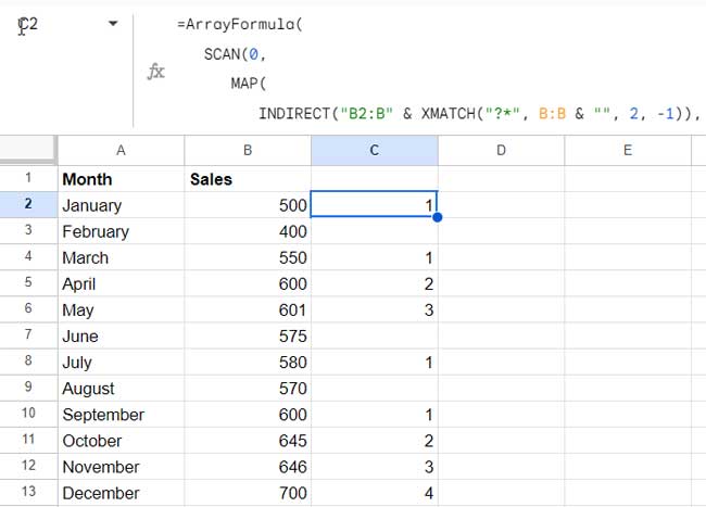
In the following example, month names are listed in column A, and corresponding sales figures are in column B. The field labels are found in A1:B1.
The data range spans from A1 to B13. Column A (A2:A13) contains month names from January to December, and Column B (B2:B13) contains sales figures in US Dollars for each respective month.
The objective is to highlight consecutive data spikes in sales.
Helper Formula:
In cell C2, enter the following array formula:
=ArrayFormula(
   SCAN(0,
      MAP(
         INDIRECT("B2:B" & XMATCH("?*", B:B & "", 2, -1)),
         LAMBDA(r, LET(pv, OFFSET(r, -1, 0), IF(r - IF(ISTEXT(pv), 0, pv)<=0, , 1)))
      ),
      LAMBDA(a, v, IF(v=0, , a+v))
   )
)
Where:
B2:Bis the specific range to evaluate for consecutive data spikes.B:Bis the column reference containing the values to be assessed.
This is a universal formula (which I will explain in a later part of this tutorial). Essentially, the formula is designed for highlighting ‘n’ consecutive data spikes. It’s important to note that you’ll need to specify the value of ‘n’ within the highlighting rule, not within this formula.

How do I interpret the result?
The formula returns sets of sequence numbers. Each set is broken by blank cells, indicating a decrease in value. If the formula returns a sequence from 1 to 3, it means there are consecutive three increases. Similarly, a sequence from 1 to 4 means there are 4 consecutive increases.
Conditional Format Rule:
Conditional Formatting for Three Consecutive Increases:
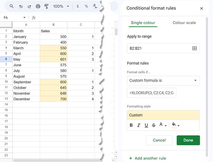
=XLOOKUP(3, C2:C4, C2:C4, , 1, -1)The formula searches for ‘n’ (3) within the ‘n’ cells (C2:C4) in the helper range and returns the value that is greater than or equal to ‘n’ (3).

Conditional Formatting for Four Consecutive Increases:
=XLOOKUP(4, C2:C5, C2:C5, , 1, -1)Conditional Formatting for Five Consecutive Increases:
=XLOOKUP(5, C2:C6, C2:C6, , 1, -1)To conditionally format ‘n’ consecutive data spikes in a column, you need to adjust the formula accordingly.
To enter the above custom formula in conditional formatting in Google Sheets, you can follow these steps:
- Select the range of cells, for example, B2:B, to which you want to apply conditional formatting.
- Click on “Format” in the top menu.
- Choose “Conditional formatting” from the dropdown menu.
- In the Conditional Format Rules panel on the right, select the drop-down menu under “Format cells if” and choose “Custom formula is.”
- Enter your custom formula into the given field.
- Click on “Done.”
Highlight Data Spikes in a Row in Google Sheets
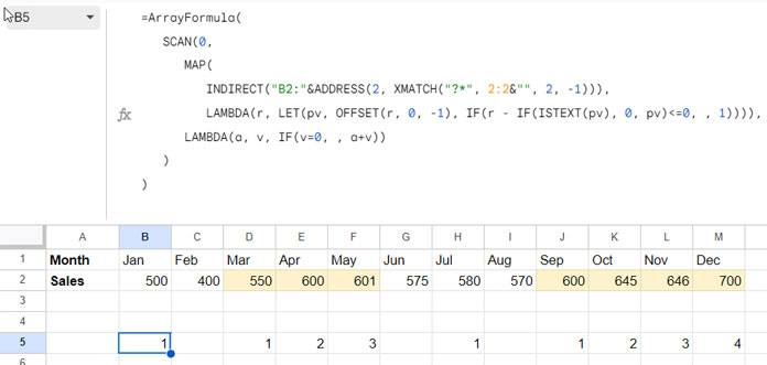
Assuming you have the month names in row #1 and sales figures in row #2.
In the sample data, A1:A2 contains the field labels Month and Sales, respectively. B1:1 contains month names, and B2:2 contains sales figures.
Here is the helper formula to find the data spike in row #2 (horizontal data):
=ArrayFormula(
   SCAN(0,
      MAP(
         INDIRECT("B2:"&ADDRESS(2, XMATCH("?*", 2:2&"", 2, -1))),
         LAMBDA(r, LET(pv, OFFSET(r, 0, -1), IF(r - IF(ISTEXT(pv), 0, pv)<=0, , 1)))
      ),
      LAMBDA(a, v, IF(v=0, , a+v))
   )
)
Where:
2:2is the row containing the sales figures to evaluate for consecutive increases.2is the row number.B2is the first cell in the range of sales figures.
You can apply this formula in column B, so I am inserting this into B5.

Highlighting Rules (pick one of the following):
=XLOOKUP(3, B5:D5, B5:D5, , 1, -1) // higlights 3 consecutive data spikes
=XLOOKUP(4, B5:E5, B5:E5, , 1, -1) // higlights 4 consecutive data spikes
=XLOOKUP(5, B5:F5, B5:F5, , 1, -1) // higlights 5 consecutive data spikes
The ‘Apply to range’ within the highlight rules must be B2:2, not A2:2.
Highlighting Consecutive Increases in a 2D Array in Google Sheets
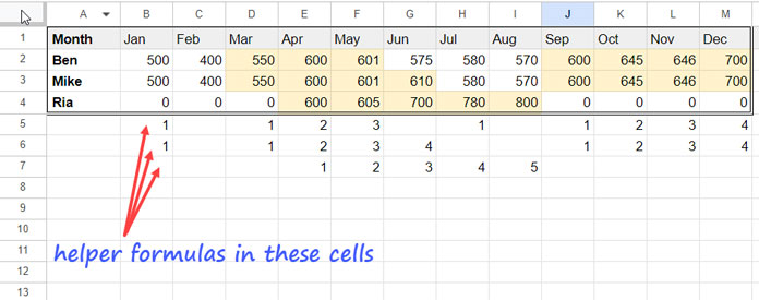
It is common to have multiple series, such as row #1 containing month names, row #2, row #3, and row #4 containing sales data for Salesperson 1, Salesperson 2, and Salesperson 3, respectively. As before, the first column, i.e., A1:A4, is dedicated to labels.
How do we highlight consecutive data spikes in rows 3 to 4?
This requires a single highlight rule, but you need multiple helper formulas to find consecutive increases in each row.

In this case, you can use the same formula found under “Highlight Data Spikes in a Row in Google Sheets” in cell B5. Copy and paste the same formula into cells B6 and B7, then replace the following parameters.
In cell B6:
2:2, the row containing the sales figures to evaluate, becomes3:3.2, row number, becomes3.B2, the first cell in the range of sales figures, becomesB3.
In cell B7, these parameters will become 4:4, 4, and B4 respectively.
Changes in the Conditional Format Rule:
In the highlight rule, the XLOOKUP formula remains the same; the only change is in the ‘Apply to range,’ which should be B2:4, not B2:2.
Note: I don’t recommend highlighting consecutive increases in a 2D array as the helper formula uses Lambda functions. They might slow down your sheet’s performance.
Understanding the Consecutive Increases Formula in Google Sheets
Let’s delve into the explanation of the formula used for the range B2:B, i.e., the column range in the first example:
=ArrayFormula(
   SCAN(0,
      MAP(
         INDIRECT("B2:B" & XMATCH("?*", B:B & "", 2, -1)),
         LAMBDA(r, LET(pv, OFFSET(r, -1, 0), IF(r - IF(ISTEXT(pv), 0, pv)<=0, , 1)))
      ),
      LAMBDA(a, v, IF(v=0, , a+v))
   )
)
Let’s break down this formula into two parts: MAP and SCAN functions parts.
MAP Function Part:
MAP(
         INDIRECT("B2:B" & XMATCH("?*", B:B & "", 2, -1)),
         LAMBDA(r, LET(pv, OFFSET(r, -1, 0), IF(r - IF(ISTEXT(pv), 0, pv)<=0, , 1)))
      ),
This follows the syntax: MAP(array1, [array2, …], lambda)
array1:INDIRECT("B2:B" & XMATCH("?*", B:B & "", 2, -1))
The formula uses XMATCH to find the last non-blank cell in column B and combines that with “B2:B” to create a closed range. INDIRECT returns values in that range to improve the overall performance of the helper formula.
Related: XMATCH First or Last Non-Blank Cell in Google Sheets
Lambda:LAMBDA(r, LET(pv, OFFSET(r, -1, 0), IF(r - IF(ISTEXT(pv), 0, pv)<=0, , 1)))
The LAMBDA function follows the syntax: LAMBDA([name, …], formula_expression).
The MAP function iterates over each value in the array1 and performs an unknown lambda function. Each value in the array is defined by ‘r’ within the LAMBDA. The function within lambda (formula_expression) subtracts the current element value (r) from the value in the cell above. The OFFSET function is employed to extract the value in the previous cell. If the output is <=0, the formula returns blank; otherwise, it returns 1.
In short, the formula returns a range with blanks or 1, where 1 denotes a spike in value.
Note: If there is any text in array1, the formula will treat it as 0. For this purpose, we use the combination of IF and ISTEXT.
To identify and highlight the consecutive data spikes in the column, we must calculate the running total of the MAP output.
SCAN Part:
SCAN(0,
      ...,
      LAMBDA(a, v, IF(v=0, , a+v))
   )
The SCAN function follows the syntax: SCAN(initial_value, array_or_range, lambda), where the initial_value is 0, and the array_or_range is the MAP output.
The Lambda uses the names ‘a’ (initial value in the accumulator, which is 0) and ‘v’ (the current element in the array), and the formula expression is IF(v=0, , a+v). In each iteration, the value is added to the accumulator, and the formula returns that intermediate calculation, resulting in a running sum.
Using XMATCH within conditional formatting enables us to highlight consecutive data spikes with the help of this running total.
Resources
This tutorial covers the following:
Highlighting data spikes (consecutive increases) in a column, row, or 2D array in Google Sheets.
I’ve covered every aspect of this highlight rule, from the formula that identifies data spikes to the highlight rule used in conditional formatting. Though this blog includes several tutorials on conditional formatting, here are some handpicked ones.
- How to Highlight Cells Based on Expiry Date in Google Sheets
- Date-Related Conditional Formatting Rules in Google Sheets
- Highlight Duplicates in Single, Multiple Columns and all Cells In Google Sheets
- Highlight Matches or Differences in Two Lists in Google Sheets
- Highlight Intersecting Value in Google Sheets in a Two-Way Lookup
- Highlight Groups When Group Total Exceeds Target in Google Sheets
- How to Highlight the Largest 3 Values in Each Row in Google Sheets


