Without mirroring values you can highlight cells in one Sheet if the same cells in another Sheet have values. This is a Google Sheets tutorial and let’s see how to do this type of cell coloring using conditional formatting in it.

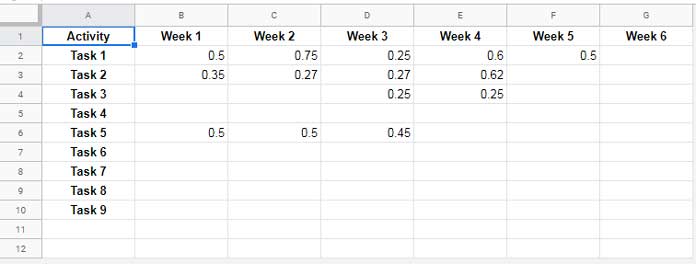
In a Google Sheets file (workbook) I have two sheets named “Sheet 1” and “Sheet 2”. In “Sheet 1” I have entered values in different columns.

I want to highlight these non-blank cells (cells with value), not in the same Sheet, but in another Sheet, i.e. in “Sheet 2”.

For this, I don’t want to mirror values because I want to keep the second Sheet entirely different. I may or may not add values in that.

Sample Data in “Sheet 1”: Consider the Values in B2:G10 for highlighting in “Sheet 2” in the same range.

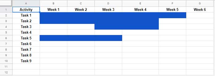
Result in “Sheet 2”: Cells in the Range B2:G10 Highlighted Based on the Values in the Same Range in “Sheet 1”.

Mirroring Sheets means to share the same values between Sheets. For example, if cell A1 in “Sheet 1” has the value 100, you can mirror that value in another Sheet using the formula = 'Sheet 1'!A1.

Let’s see how to highlight cells in “Sheet 2” based on the values (non-blank cells) in another sheet (“Sheet 1” here) in Google Sheets.

How To Highlight Cells in One Sheet if the Same Cells in Another Sheet Have Values

I have already shown you the sample data and my expected output. Now what you want is the formula to color cells based on values in another Sheet.

In the above example, I have considered the values in a particular range. But if you wish, you can include the entire Sheet.

For this, you do not need to make any changes in my formula. I’ll explain that below.

Here is the formula to highlight cells in “Sheet 2” if the same cells in “Sheet 1” have values.

=NOT(ISBLANK(INDIRECT("Sheet 1!"&Address(Row(),Column(),))))

Entering a Custom Formula in Conditional Formatting – Steps

As a side note, the above is one custom rule formula for conditional formatting. Similarly, you can use custom formula rules in Data Validation and Filter. Want to see examples to custom formula rule in the Filter Menu command? Here you go!

1. How to Filter by Month Using the Filter Menu in Google Sheets.
2. Filter Unique Values Using the Filter Menu in Google Sheets.

To apply custom formula rule in Google Sheets conditional formatting, follow the below few steps.

1. Go to “Sheet 2” since we want to color cells in this Sheet.
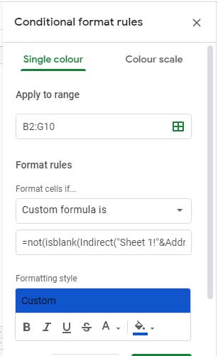
2. Click the menu “Format” and choose Conditional formatting...
3. Enter B2:G10 in the field under Apply to range. Please note that the same range in “Sheet 1” will only be considered in “Sheet 2” for highlighting. That means here you can control the range to highlight. If you want to highlight an entire Sheet, just enter the range A1:1000 (1000 rows) in the said field.
4. Use the above-provided formula below the Custom formula is field.

If the above settings confuse you, see the below screenshot.

Follow the above tips to highlight cells if the same cells have values in another Sheet in Google Sheets.

More Conditional Formatting Tips:

1. How to Conditional Format a Chessboard in Google Sheets.
2. Find All the Cells Having Conditional Formatting in Google Sheets.
3. Compare Two Google Sheets Cell by Cell and Highlight.
4. Highlight Matches or Differences in Two Lists in Google Sheets.
5. How to Conditional Format Duplicates Across Sheet Tabs in Google Sheets.