Google Sheets: Highlight Cells if Same Cells in Another Sheet Have Values

You can highlight cells in one sheet based on whether the same cells in another sheet have values, and you don’t even need to mirror the data. Here’s how to highlight cells if the same cells in another sheet have values without duplicating data.

In this Google Sheets tutorial, you’ll learn how to apply conditional formatting that references another sheet to highlight matching non-blank cells.

Table of Contents

Scenario Overview

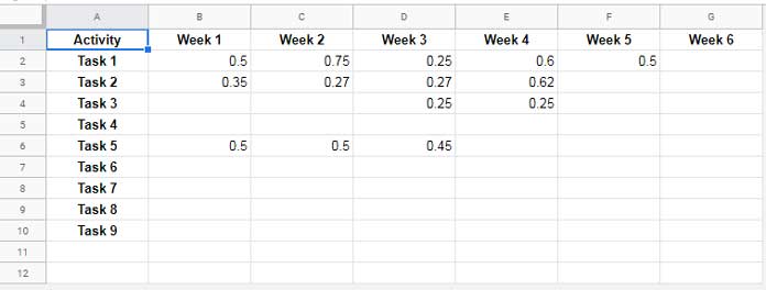
Suppose you have two sheets in your Google Sheets file:

Sheet1: Contains the original values
Sheet2: You want to highlight cells here if the same cell in Sheet1 has a value

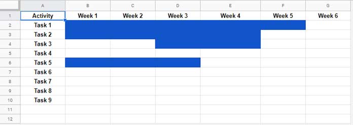
Let’s say the range B2:G10 in Sheet1 contains various entries, and you want to highlight the same cell positions in Sheet2 only if there’s a value in Sheet1.

Example Setup

Sheet1’s Data:

Sample job schedule in Sheet1 used to highlight same cells in another sheet without mirroring data in Google Sheets

Sheet2’s Highlighting Result:

Highlighted cells in Sheet2 based on values in the same cells of Sheet1 in Google Sheets

Why Not Mirror the Data?

You could mirror cells using formulas like ='Sheet1'!B2, but that would overwrite Sheet2’s content and structure. This method highlights cells without changing or duplicating any data in Sheet2.

How to Highlight Cells by Another Sheet’s Data

Step 1: Use This Conditional Formatting Formula

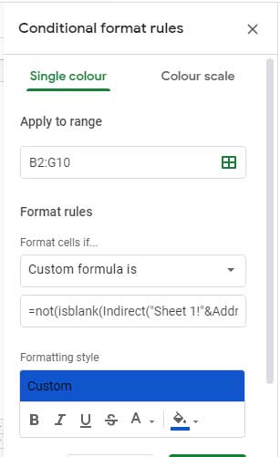
=NOT(ISBLANK(INDIRECT("Sheet1!" & ADDRESS(ROW(), COLUMN()))))

What it does:

ROW() and COLUMN(): Refer to the current cell’s position
ADDRESS(...): Builds a string like "B2"
INDIRECT(...): Accesses that address in Sheet1
ISBLANK(...): Checks if the referenced cell is empty
NOT(...): Returns TRUE when the referenced cell has a value

Step 2: Apply Conditional Formatting

Go to Sheet2
Select the range you want to highlight (e.g., B2:G10)
Click Format > Conditional formatting
Under Apply to range, enter B2:G10
Under Format cells if, choose Custom formula is
Paste the formula from Step 1
Pick a fill color
Click Done

Applying a conditional formatting rule in Google Sheets to highlight cells based on another sheet’s data

Cells in Sheet2 will now be highlighted if the same cell in Sheet1 contains any value.

Optional: Highlight an Entire Sheet

If you’d like to highlight the entire Sheet2 (e.g., up to 1000 rows), set the Apply to range to A1:1000.
The formula still works for each cell individually.

Example Use Case

Let’s say you maintain job schedules or attendance records across multiple tabs.
This method helps you visually track updates in the source sheet without duplicating any values.

Final Tip

You’re not limited to just non-blank cells—you can customize the formula to highlight based on specific values, text, or even patterns from another sheet.

This approach is ideal when you want to highlight cells in one sheet based on values in another, without disrupting layout or content.