How to Generate Random Groups in Google Sheets

Google Sheets is a powerful tool for generating random groups from any set of members. This is useful in many real-life scenarios, such as selecting equal-sized data for sampling, creating teams, randomly allocating jobs to groups, etc.

You don’t need to rely on drag-down formulas in Google Sheets, as this can be easily accomplished with a combination of array formulas such as SEQUENCE, RANDARRAY, and SORT.

In the following example, we have 12 players for 3-on-3 basketball. Let’s see how to group them into 4 groups of 3 players each randomly. It’s easy to customize the formula to adjust both the number of players in each group and the total number of players.

Since the formula uses the volatile RANDARRAY function, the groups will be shuffled whenever changes are made to the sheet and at specific recalculation settings such as every minute or hour.

I’ll also cover how to generate static random groups in Google Sheets and how to filter them at the end of this tutorial.

Step 1: Creating a New Sheet and Adding Player Names

In a new Google Sheets file, enter the names for random grouping into column A (starting from A2, with A1 reserved for the column header). You can quickly create a new sheet by clicking https://sheet.new/

Step 2: Assigning Sequence Numbers

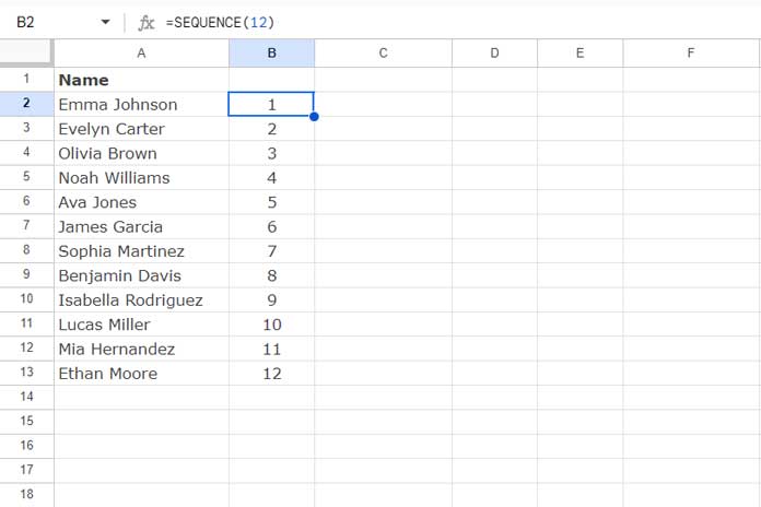
Formula for Assigning Sequence Numbers to Player Names

In cell B2, enter the following SEQUENCE formula to generate sequence numbers from 1 to 12:

=SEQUENCE(12)

If you have more players, such as 20, replace 12 with 20 in the formula.

Step 3: Dividing Sequence into Groups for Randomization

Dividing Sequence Numbers into Groups for Randomization

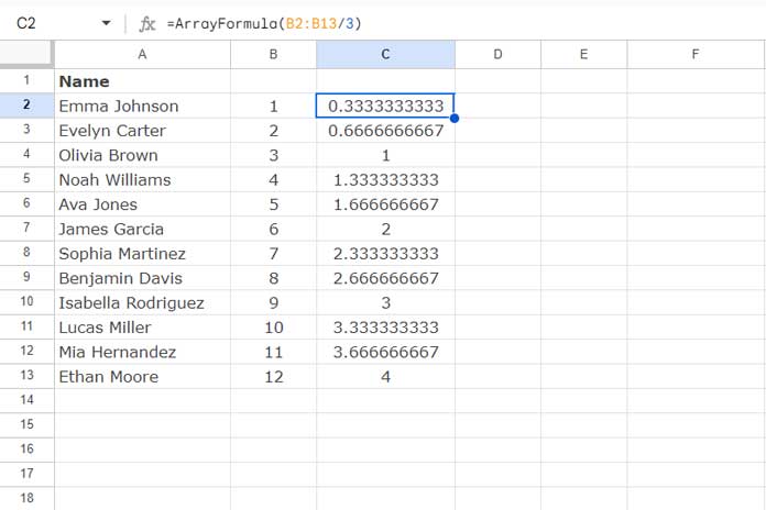
This step determines the number of players in each group. We are creating random groups of 3 players each.

Enter the following formula in cell C2:

=ArrayFormula(B2:B13/3)

If you want to generate groups of 5 players each, replace 3 with 5 in the formula.

Step 4: Rounding Up the SEQUENCE Values

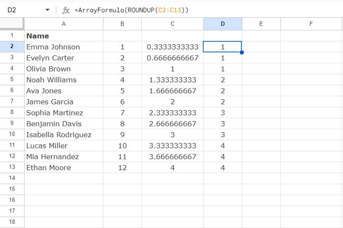
By rounding up the results from Step 3, you will group players into sets of 3 in a sequence. To round up, use the following formula in cell D2:

=ArrayFormula(ROUNDUP(C2:C13))

In the next step, we will randomize these group numbers to generate random groups of players.

Step 5: Generating Random Groups

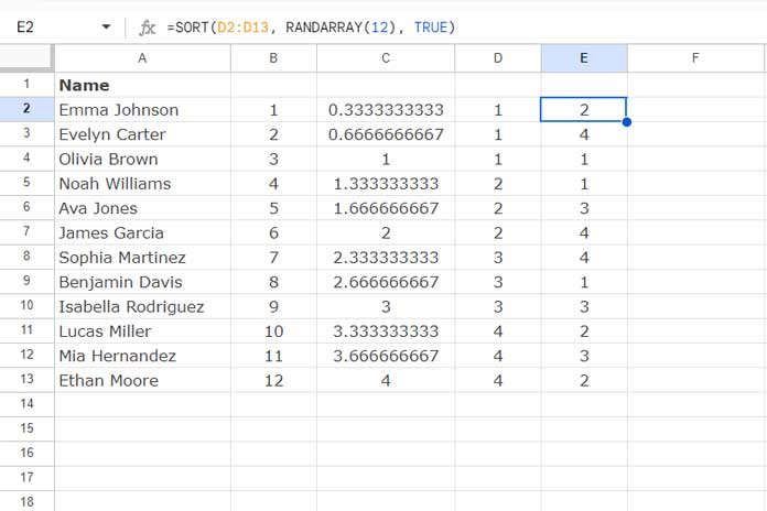
Formula for Generating Random Groups of Players

In cell E2, enter the following formula to randomly shuffle the groups of 3 players each:

=SORT(D2:D13, RANDARRAY(12), TRUE)

If you have more players, replace 12 in the formula to match your total number of players. Also, replace D2:D13 with the range reference to include those names.

Here’s how it works:

SORT(D2:D13, RANDARRAY(12), TRUE): This formula sorts your groups from D2:D13 using 12 random numbers generated by RANDARRAY. It shuffles the groups based on these random numbers.
RANDARRAY(12) creates 12 random numbers, which the SORT function uses to mix up the order of the groups.

This is how to generate random groups in Google Sheets.

Creating Static Random Groups

The formula above has one significant drawback: it reshuffles the groups every time there’s a change in the sheet or at specific time intervals (check the Calculation settings by clicking File > Settings).

This means you might not be able to filter or work with the groups consistently using the FILTER or other functions.

To create static random groups that only refresh when you choose, you can use the following formula in cell E2 as a replacement for Step 5:

=LAMBDA(srt, SORT(D2:D13, srt, TRUE)) (RANDARRAY(12))

To refresh the grouping, simply copy this formula from cell E2, delete the formula in E2, and paste it back. This way, you get a new random grouping only when you decide to refresh it.

Here’s how it works:

LAMBDA creates a custom function to sort your groups.
RANDARRAY() generates a random array just once when the formula is initially calculated. This ensures that the random numbers stay fixed.
The result of RANDARRAY() is passed to the LAMBDA function, which uses it to sort the groups. Since it’s a one-time calculation, the values don’t change unless you manually update them.

Note: This method is not 100% foolproof. I’ve noticed that it can lose its static behavior in two instances: when you first close and reopen the file, or when you delete all rows below and to the right of the last row of the random group.

Creating Random Groups without Helper Cells

If you have names in A2:A13 and want to generate groups directly in B2:B13 using a single formula, you can use the following approach:

For a formula that automatically updates when you make changes to your sheet, use:

=SORT(ROUNDUP(SEQUENCE(12)/3), RANDARRAY(12), TRUE)

Replace 12 with the total number of members and 3 with the number of members you want in each group.

If you prefer a static version that only refreshes when you manually update it, use:

=LAMBDA(srt, SORT(ROUNDUP(SEQUENCE(12)/3), srt, TRUE))(RANDARRAY(12))

This will keep your groups static until you choose to refresh them, as mentioned earlier.

Filtering and Displaying Generated Random Groups

Generate Random Groups and Filter the Names

If you want to filter names into new ranges based on their random group, you should use the static random group formula from above.

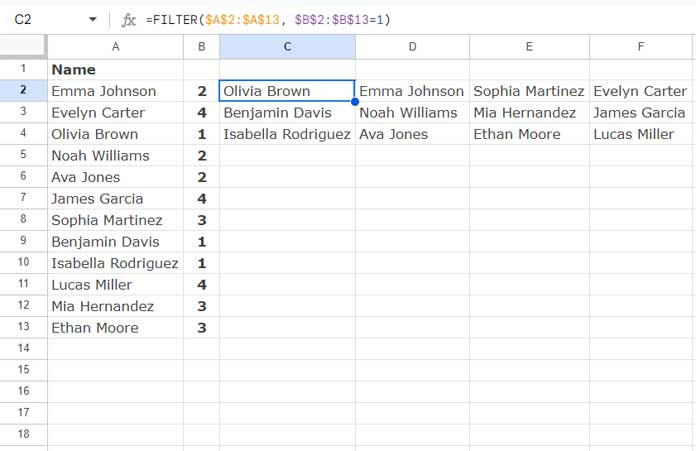
Assuming the static random group formula is in place in cell B2, you can use the following FILTER formula in cell C2 to display the first group of players:

=FILTER($A$2:$A$13, $B$2:$B$13=1)

To filter the other groups, enter similar formulas in cells D2, E2, and F2, replacing the number 1 with 2, 3, and 4, respectively.