")
")


")


")

")
")
 in Excel & Google Sheets")


You can insert group total rows in your dataset without using LAMBDA functions or any performance-affecting formula in Google Sheets. This approach is efficient and helps you handle very large datasets without issues.
Introduction
What does it mean to insert group total rows in Google Sheets?
When you have category-wise data related to sales, purchases, expenses, or other categories, inserting group total rows can help summarize the data more effectively.
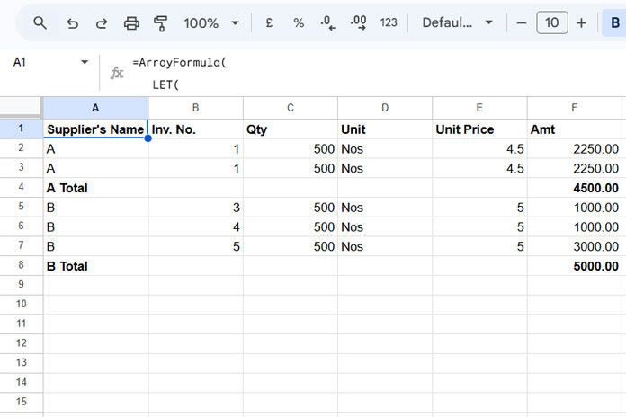
For example, consider the following accounts payable data for materials purchased from different vendors:
| Supplier’s Name | Inv. No. | Qty | Unit | Unit Price | Amt |
| A | 1 | 500 | Nos | 4.5 | 2250.00 |
| A | 1 | 500 | Nos | 4.5 | 2250.00 |
| B | 3 | 500 | Nos | 5 | 1000.00 |
| B | 4 | 500 | Nos | 5 | 1000.00 |
| B | 5 | 500 | Nos | 5 | 3000.00 |
You can insert a total row below each supplier (e.g., A, B) to easily calculate the total outstanding payable amount for each vendor.
With the formula provided in this tutorial, you don’t need to sort the data based on the group column (e.g., the supplier’s name). The formula will handle it automatically.
Formula to Insert Group Total Rows in Google Sheets
Assume the above sample data is in Sheet1 of your Google Sheets file. You can use the following formula in cell A1 of Sheet2:
=ArrayFormula(
   LET(
      cat, UNIQUE(TOCOL(Sheet1!A2:A, 1)),
      amt, SUMIF(Sheet1!A2:A, cat, Sheet1!F2:F),
      catAmt, IFNA(HSTACK(cat&" Total","", "", "", "", amt)),
      alldata, VSTACK(Sheet1!A1:F, catAmt),
      QUERY(alldata, "SELECT * WHERE Col1 IS NOT NULL ORDER BY Col1", 1)
   )
)
Adjustments for Your Data
In this formula, it is assumed that the first column represents the category column and the last column represents the amount column.
When applying this formula to your dataset, make the following changes:
- Replace
Sheet1!A2:Awith the range reference of the category column (the first column). - Replace
Sheet1!F2:Fwith the range reference of the amount column (the last column).
Note: These references exclude the header row.
- Replace
Sheet1!A1:Fwith the reference to the entire dataset, including the header row.
Key Section of the Formula:
HSTACK(cat & " Total", "", "", "", "", amt)The "", "", "", "" (four empty strings) represent padding for the blank columns between the category and amount columns. Adjust the number of empty strings based on the structure of your dataset.
Inserting Group Totals Rows When the Amount Column Is Not the Last Column
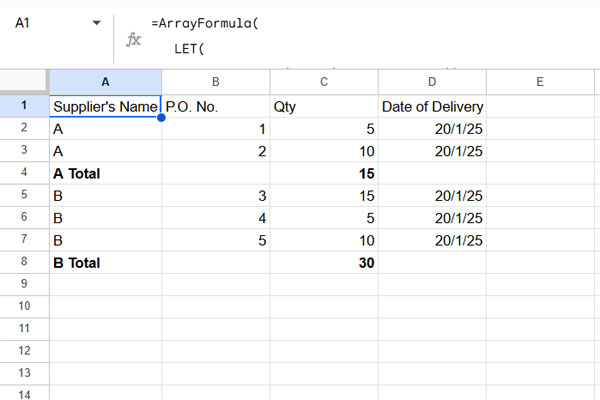
Sample Data (Sheet3):
| Supplier’s Name | P.O. No. | Qty | Date of Delivery |
| A | 1 | 5 | 20/1/25 |
| A | 2 | 10 | 20/1/25 |
| B | 3 | 15 | 20/1/25 |
| B | 4 | 5 | 20/1/25 |
| B | 5 | 10 | 20/1/25 |
In the sample data above, the category column is the first column (Supplier’s Name), but the amount column (the column to total) is the third column (Qty), not the last column (Date of Delivery). Here’s how you can adjust the formula to insert the group total rows.
Updated Formula:
=ArrayFormula(
   LET(
      cat, UNIQUE(TOCOL(Sheet3!A2:A, 1)),
      amt, SUMIF(Sheet3!A2:A, cat, Sheet3!C2:C),
      catAmt, IFNA(HSTACK(cat&" Total", "",amt, "")),
      alldata, VSTACK(Sheet3!A1:D, catAmt),
      QUERY(alldata, "SELECT * WHERE Col1 IS NOT NULL ORDER BY Col1", 1)
   )
)
Inserting Group Totals Rows When the Category Column Is Not the First Column
Sample Data (Sheet5):
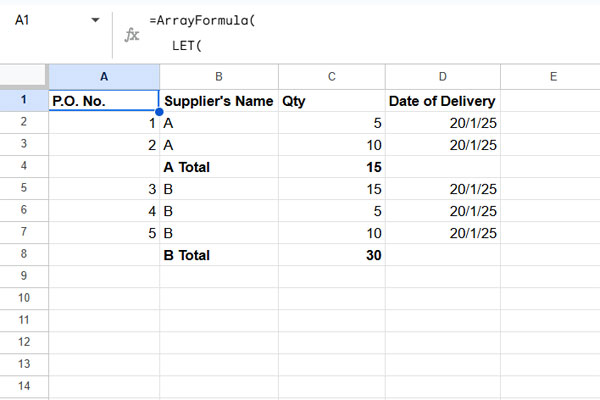
If your category column is not the first column, you need to modify the QUERY part to reference the correct column. For example, consider the following sample data where the category column is the second column:
| P.O. No. | Supplier’s Name | Qty | Date of Delivery |
| 1 | A | 5 | 20/1/25 |
| 2 | A | 10 | 20/1/25 |
| 3 | B | 15 | 20/1/25 |
| 4 | B | 5 | 20/1/25 |
| 5 | B | 10 | 20/1/25 |
In this case, you should modify the QUERY as follows:
QUERY(alldata, "SELECT * WHERE Col2 IS NOT NULL ORDER BY Col2", 1)Additionally, you need to adjust the padding in the HSTACK function (i.e., HSTACK("", cat & " Total", amt, "")) to match the structure of your dataset.
Formula:
=ArrayFormula(
   LET(
      cat, UNIQUE(TOCOL(Sheet5!B2:B, 1)),
      amt, SUMIF(Sheet5!B2:B, cat, Sheet5!C2:C),
      catAmt, IFNA(HSTACK("", cat&" Total", amt, "")),
      alldata, VSTACK(Sheet5!A1:D, catAmt),
      QUERY(alldata, "SELECT * WHERE Col2 IS NOT NULL ORDER BY Col2", 1)
   )
)
Formula Explanation
Let’s break down the last formula step by step:
- cat:
UNIQUE(TOCOL(Sheet5!B2:B, 1))
Extracts unique categories, excluding empty cells.
- amt:
SUMIF(Sheet5!B2:B, cat, Sheet5!C2:C)
Calculates the group totals for each category.
- catAmt:
IFNA(HSTACK("", cat&" Total", amt, ""))
Combines categories and totals while padding empty columns.
- alldata:
VSTACK(Sheet5!A1:D, catAmt)
Combines the source data and group total rows.
- Final QUERY Expression:
QUERY(alldata, "SELECT * WHERE Col2 IS NOT NULL ORDER BY Col2", 1)
Removes empty rows and sorts the categories in ascending order.
Conclusion
This formula provides a resource-friendly way to insert group totals in Google Sheets. Here’s why it’s efficient:
- It doesn’t use LAMBDA functions, avoiding iterative calculations.
- It processes only unique categories rather than entire columns, making it faster and less prone to errors in large datasets.
By following this approach, you can easily and efficiently manage grouped totals in your datasets.
What if I have multiple columns to total, such as a quantity column and an amount column?
In such cases, refer to the first tutorial listed under the resources below.
Resources
- Insert Subtotal Rows in a Google Sheets Query Table
- Reset Running Total at Blank Rows in Google Sheets
- Group and Sum Data Separated by Blank Rows in Google Sheets
- Grouping and Subtotal in Google Sheets and Excel
- AT_EACH_CHANGE Named Functions in Google Sheets
- Dynamic Total Row for FILTER, QUERY, or ARRAY Results in Sheets
- Calculate Subtotals Up to the First Blank Cell in Google Sheets
This is an excellent tutorial!
I really appreciate how you went through each of the steps. So I could understand what is happening behind the scenes.
I am trying to take this one step further and provide totals on an additional column.
I’m wondering if you could look at my work and let me know if what I want to do is possible?
I’ve placed my work in the following Sheet: — address removed by admin —
Hi, Todd Powers,
Please see my comment in cell C1 in your sheet for the formula and notes.
That formula is based on another tutorial – Inserting Subtotal Rows in a Query Table in Google Sheets.
Very Informative , Very Well Explained
This is excellent. Without Google Apps Script, but with just 2 formulas, the output is great. However, can we have the Total row first and then the details row. Please let us know.
Hi, Abraham,
In Query change
order by Col1 asctoorder by Col1 desc.This may do the trick.