


")


")

")
")
 in Excel & Google Sheets")


You don’t need to use QUERY or FILTER to extract the last entry of each item by date in Google Sheets. Instead, you can use a simple combination of SORT and SORTN.
The SORT function is unnecessary if your data is already sorted by the item column and then by the date column. However, for flexibility, we will include it. This formula extracts the latest records from each group based on the date entries.
Where Is This Useful?
Extracting the last entry of each item by date in Google Sheets is useful in various real-life scenarios, such as:
- Tracking the last recorded stock update for each product.
- Finding the latest PO (purchase order) for each customer.
- Extracting the most recent payment or invoice details.
- Tracking the most recent leave request per employee/student.
- Extracting the most recent status change for ongoing projects.
Generic Formula
=SORTN(SORT(range, key_col, TRUE, dt_col, FALSE), 9^9, 2, key_col, TRUE)Where:
range– The data range containing the records.key_col– The column number determining the grouping (e.g., product name column number, employee name column number).dt_col– The column number containing the date entries.
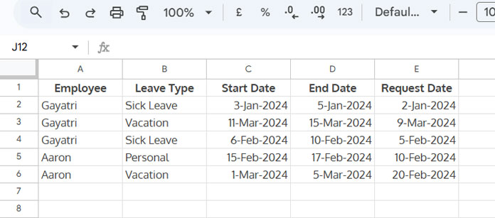
Example 1: Extracting the Last Leave Request for Each Employee
Consider the following employee leave data:
To extract the last leave request record for each employee:
key_colis column A (Employee Name).dt_colis column E (Leave Request Date).
Formula:
=SORTN(SORT(A2:E, 1, TRUE, 5, FALSE), 9^9, 2, 1, TRUE)Output:
| Employee | Leave Type | Start Date | End Date | Request Date |
| Aaron | Vacation | 1-Mar-2024 | 5-Mar-2024 | 20-Feb-2024 |
| Gayatri | Vacation | 11-Mar-2024 | 15-Mar-2024 | 9-Mar-2024 |
How This Works:
SORT(A2:E, 1, TRUE, 5, FALSE): Sorts data by employee name (ascending) and then by request date (descending).- This ensures that each employee’s latest leave request appears first in their group.
SORTN(..., 9^9, 2, 1, TRUE): Removes duplicate rows based on employee names, keeping only the latest record per employee.
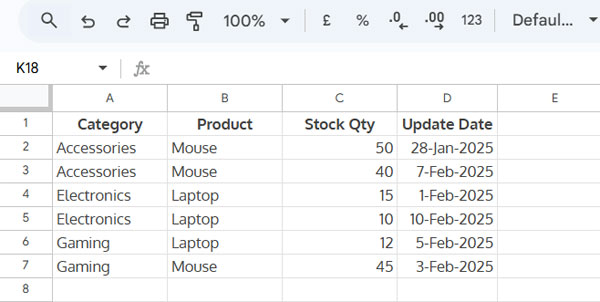
Example 2: Extracting the Last Stock Update per Product
Here is sample data for tracking the last recorded stock update for each product:
To extract the last entry of each Product by date:
=SORTN(SORT(A2:D, 2, TRUE, 4, FALSE), 9^9, 2, 2, TRUE)Output:
| Category | Product | Stock Qty | Update Date |
| Electronics | Laptop | 10 | 10-Feb-2025 |
| Accessories | Mouse | 40 | 7-Feb-2025 |
To extract the last updated date by Category:
=SORTN(SORT(A2:D, 1, TRUE, 4, FALSE), 9^9, 2, 1, TRUE)Output:
| Category | Product | Stock Qty | Update Date |
| Accessories | Mouse | 40 | 7-Feb-2025 |
| Electronics | Laptop | 10 | 10-Feb-2025 |
| Gaming | Laptop | 12 | 5-Feb-2025 |
To extract the last updated date by Category and then by Product:
=SORTN(SORT(A2:D, 1, TRUE, 2, TRUE, 4, FALSE), 9^9, 2, 1, TRUE, 2, TRUE)Output:
| Category | Product | Stock Qty | Update Date |
| Accessories | Mouse | 40 | 7-Feb-2025 |
| Electronics | Laptop | 10 | 10-Feb-2025 |
| Gaming | Laptop | 12 | 5-Feb-2025 |
| Gaming | Mouse | 45 | 3-Feb-2025 |
Conclusion
This tutorial demonstrated how to extract the last entry of each item by date in Google Sheets using SORT and SORTN. These formulas help efficiently retrieve the most recent records in various scenarios.
Hi Prashanth 😊
I need to pull out every last data for every end of the month in C9, C16, C20. thank you.
Hi, Bahar,
Thanks for the sheet link.
We can’t use the formula mentioned in this tutorial to solve the problem. I’ll come back to you with a new tutorial soon.
Hi, Bahar,
I have inserted the formula into your sheet.
Here you can find the explanation and an alternative formula too.
Return Month End Rows from Daily Data in Google Sheets.