You can find the second-highest value from each group in Google Sheets with an array formula.
First, let’s see how to find the second-highest value in a column. For example, to find the second-highest salary in column B, use the following formulas:
- Without Removing Duplicates:
=LARGE(B:B, 2)- After Removing Duplicates:
=LARGE(UNIQUE(B:B), 2)In the first example, we used the LARGE function directly on column B. In the second example, we applied the LARGE function to the unique values in column B.
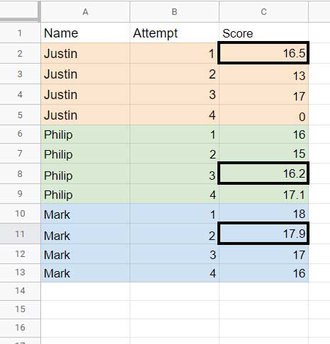
Now, consider a table with student scores from a sports event. Column A contains student names, Column B shows their attempt numbers (1-4), and Column C lists their scores.

To extract the second-highest score for each student from this table:
- Sort Data: Sort Column A (Names) in ascending order and Column C (Scores) in descending order.
- Running Count: Use COUNTIFS to find the running count of occurrences for each name in Column A.
- Filter Results: Filter the sorted data to keep only the rows where the running count equals 2.
We’ll combine these steps into a single formula to find the second-highest value from each group in Google Sheets. Let’s dive in!
Formula to Find the Second Highest Value in Each Group
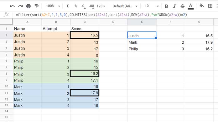
For the above sample data, we can use the below combination formula.
=FILTER(
     SORT(A2:C, 1, 1, 3, 0),
     COUNTIFS(SORT(A2:A), SORT(A2:A), ROW(A2:A), "<="&ROW(A2:A))=2
)
Note:
To find the third highest value, you can change the criterion =2 to =3 in the formula. Similarly, you can modify the formula to return the nth highest value in each group.
If you want to return all values up to the 2nd highest, you can adjust the formula by changing =2 to <=2.
This approach can also be applied to date or timestamp columns instead of numeric values.
Can You Split this Formula and Explain?
Yes! Here’s an explanation of the formula.
The formula has three main steps: Sort, Countifs, and Filter.
Step 1: Sorting the Data
Let’s start by understanding what the SORT formula does. For explanation purposes, I’ve split the original formula and inserted the components into individual cells.
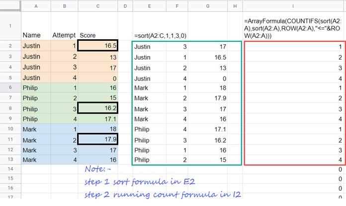
In cell E2, the SORT formula:
=SORT(A2:C, 1, 1, 3, 0)This sorts the names in ascending order (Column A) and the scores in descending order (Column C). As a result, names appear in alphabetical order, and the highest scores are at the top. (Refer to columns E to G in the image below.)

Step 2: Creating a Running Count
Next, in cell I2, the COUNTIFS formula:
=ArrayFormula(COUNTIFS(SORT(A2:A), SORT(A2:A), ROW(A2:A), "<=" & ROW(A2:A)))This formula generates a running count of sorted names, providing a count of each occurrence. (See column I in the image above.)
Step 3: Filtering for the Second Highest Value
Finally, the third step is to filter the data to find the second-highest score in each group.
The generic formula for this step is:
=FILTER(step_1, step_2=2)This FILTER formula extracts the rows from Step 1 where the running count from Step 2 equals 2, thus finding the second highest value in each group.
Second Largest Values in Each Group, Skipping Duplicates
In the source data above, let’s assume that Mark’s (a name in column A) scores are as follows (others’ scores remain the same):
| 18 |
| 17.9 |
| 16 |
| 18 |
According to our earlier formula, the second largest value would be 18 because the highest value, 18, repeats twice.
What if I Want to Skip Duplicates?
To skip duplicates, assume the source data is in A1:C on a tab named ‘Data’. In a new tab named ‘Result’, use the following SORTN formula in cell A2:
=SORTN(Data!A2:C, 9^9, 2, 1, 1, 3, 0)Then, apply our earlier formula from Data!E2 in cell E2 on the ‘Result’ tab to get the correct result.
Note: This method has one limitation. If all the scores in a group are the same (e.g., if all of Mark’s scores are 18), the result won’t show the second-highest score for Mark.
As mentioned earlier, you can use the same formula on a date or timestamp column instead of a number column to find the second-largest date or timestamp in each group.
That’s all about how to find the second-highest value in each group from a table or list in Google Sheets.


