


A combination of Vlookup and Match or Xmatch is the best way to find the product price based on quantity in Google Sheets.
All other combinations may require the help of a LAMBDA helper function to expand (spill) down. I’ll include one such solution too in this tutorial for educational purposes.
Assume you run an office supplies store, and you have multiple prices to offer based on order quantity.
For example, you sell a “Pen” for $2.00, and if the order quantity is 10, you sell it for $1.25 per “Pen.”
In such cases, you can prepare a price table in Google Sheets and use my array formula to find the product prices based on their order quantities.
In the following example, the price table is in the range B2:G6. Ignore B1:G1, as it contains some notes for your reference.
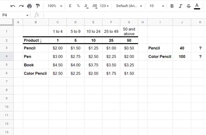
A customer ordered 40 pencils and 100 colored pencils. You can find that data entered in I3:J4.
Their unit price must be $1.00 and $1.50, respectively.
We can use an array formula in cell K3 to get those products’ prices based on quantities in Google Sheets.
Vlookup and Match for Finding Product Price Based on Quantity (Array Formula)
We will start with the VLOOKUP and MATCH combination, and here is the generic formula.
=ArrayFormula(ifna(vlookup(ordered_item,table,match(ordered_qty,table_first_row,1),0)))In this generic formula, ordered_item, ordered_qty, table, and table_first_row are the names (identifiers).
We must replace them with corresponding cell or array references in the formula expression.
Let’s understand them one by one first.
ordered_item: The cell or array that contains the product names to search in the table for the price (I3:I4).
ordered_qty: Quantity corresponding to ordered_item (J3:J4).
table: The price table (B2:G6).
table_first_row: It’s the first row of the table (A2:G2).
As per the above, we can use the below formula to find the product (I3:I4) price based on quantity (J3:J4).
Formula # 1 (Insert in K3, but empty K3:K4 beforehand for the formula # 1 to spill down):
=ArrayFormula(ifna(vlookup(I3:I4,B2:G6,match(J3:J4,B2:G2,1),0)))In the above formula, we can replace Match with XMATCH, and here it is.
Alternative:
=ArrayFormula(ifna(vlookup(I3:I4,B2:G6,xmatch(J3:J4,B2:G2,-1),0)))Index, Match, and Map for Finding Product Price Based on Quantity (Array Formula)
Here is another array formula that uses an INDEX and Match combination.
It is just for educational purposes. I suggest you use the Vlookup and Match combo (Formula # 1) above.
The purpose of the MAP lambda here is to expand the result of the Index and Match, which is not expandable otherwise.
Here also, we will consider the price table (sample) of an office supplies store.
Generic Formula:
=map(ordered_item,ordered_qty,lambda(a,b,ifna(index(table,match(a,table,0),match(b,table_first_row,1)))))Just replace the names in the formula expression with corresponding arrays.
Formula # 2 (Insert in K3, but empty K3:K4 beforehand for the formula # 2 to spill down):
=map(I3:I4,J3:J4,lambda(a,b,ifna(index(B2:G6,match(a,B2:B6,0),match(b,B2:G2,1)))))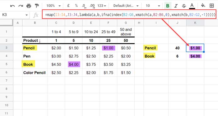
Since we have used the same names (identifiers) defined in formula # 1, I’m not explaining the same here.
Here also, we can replace Match with Xmatch to find the product price based on quantity.
Alternative:
=map(I3:I4,J3:J4,lambda(a,b,ifna(index(B2:G6,xmatch(a,B2:B6,0),xmatch(b,B2:G2,-1)))))Formula Logic in General
Both of the above Google Sheets formulas may seem complex to some of you.
Let me simplify them for you.
Formula # 1:
To return the price of the “Pencil” for quantity 40, we can use the following Vlookup and Match formula.
=vlookup("Pencil",B2:G6,match(40,B2:G2,1),0)The Vlookup searches “Pencil” and returns the price from the Match column.
We have used ARRAYFORMULA to expand this result.
Formula # 2:
To return the price of the “Pencil” for quantity 40, we can use the following Index-Match formula.
=index(B2:G6,match("Pencil",B2:B6,0),match(40,B2:G2,1))The Index offsets rows and columns returned by the Match formulas within.
We have used Map to expand this result.
That’s all about how to find the product price based on quantity in Google Sheets.
Thanks for the stay. Enjoy!