


I’ll begin by outlining the scenario before delving into the formula for finding a specific previous day from a date cell in Google Sheets.
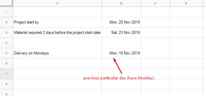
Imagine you’re in charge of a construction site, gearing up to kick off a project with a scheduled start date, let’s say, on the 25th of November 2019.
To ensure everything runs seamlessly, you need to arrange the required materials two days before the project’s commencement directly at the site. The twist? The material delivery truck operates exclusively on Mondays.
Here’s the challenge: How do you pinpoint the last Monday before your project start date minus two days? This way, you can ensure that the materials are on-site in advance, well before the project officially begins.
Recently, one of my readers presented a similar scenario, prompting this Google Sheets tutorial.
In this guide, I’ll walk you through a formula to find a specific previous day from a date cell. Specifically, we’ll tackle how to identify the last occurrence of weekdays or weekends based on a given date.
So, whether you’re searching for the last Saturday, Friday, Thursday, Wednesday, Tuesday, Monday, or Sunday relative to a date in a cell, my formula has you covered. Let’s dive in!
Example: Finding the Last/Previous Specific Day from a Date Cell
The project start date, located in cell B2, is set as Monday, 25th November 2019, for the purpose of this example. While you can use any date, I’ll be deducting 2 days from this date in cell B3 using the formula =B2-2, resulting in Saturday, 23rd November 2019.
Following the scenario outlined earlier, you have the option to skip the project start date in cell B2 and directly focus on finding a specific previous day from the date in cell B3.
The formula I’m about to share centers around the date in cell B3. Feel free to disregard the project start date.
Let’s find the last Monday, denoted as Monday, 18th November 2019, using a formula derived from the date in cell B3.
Keep in mind that you can effortlessly modify the formula to find any other day of the week or weekend. I’ll provide a tip for that as well.
Essential Functions for Finding a Specific Previous Day in Google Sheets
To find the previous day (specifically Monday) from the date in cell B3, we need two essential Google Sheets functions: WEEKDAY and IF.
- WEEKDAY: This function helps determine the weekday from the date in cell B3. If you’re new to this date function and eager to explore more, check out our comprehensive tutorial: How to Utilize Google Sheets Date Functions (Complete Guide).
- IF: This function plays a crucial role in identifying a particular previous day based on the date in cell B3. The formula’s intricacies involving the IF function will be explained in detail below.
If you want to master the IF function and explore its advanced applications, don’t miss our tutorial: How to Use the IF Function in Google Sheets (Advanced Tips).
Furthermore, we’ll incorporate the LET function to streamline the formula, making it more readable, easier to edit, and improving overall performance.
Formula to Find Specific Previous Day in Google Sheets
The following formula retrieves the specific weekday (in this case, Monday) from the provided date in cell B3.
=LET(
   dt, B3,
   wd, WEEKDAY(dt),
   twd, 2,
   IF(wd>twd, dt-wd+twd,
      IF(wd<twd, dt-7-wd+twd,
         dt-7
      )
   )
)
When employing this formula, ensure to make two adjustments. Substitute B3 with the cell containing your source date and replace 2 with the weekday number corresponding to your desired previous date. Weekday numbers range from 1 to 7, representing Sunday to Saturday.
Step-by-Step Formula Construction: Understanding the Formula
Allow me to guide you through the formulation process step by step, making it easy for you to code later.
For the time being, we’ll utilize two helper cells, namely C3 and D3. Keep in mind that these references to the helper cells will be eliminated from the formula at a later stage.
Cell C3: Weekday Number Calculation
Using the WEEKDAY function, determine the weekday number of the date in cell B3.
=WEEKDAY(B3)This function will yield 7 since Saturday (23/11/2019) holds a weekday number of 7 in a week starting from Sunday and ending on Saturday.
Weekday Numbers:
- Sunday – 1
- Monday – 2
- Tuesday – 3
- Wednesday – 4
- Thursday – 5
- Friday – 6
- Saturday – 7
Cell D3: Set Target Weekday Number
Enter 2 in cell D3, corresponding to the weekday number of Monday. This value will be utilized to find the last occurrence of the specified weekday, i.e., Monday, from the date in cell B3.
This tutorial focuses on uncovering a specific previous day, not necessarily Monday. Adjust the value in D3 accordingly; for instance, input 4 to find the last Wednesday.
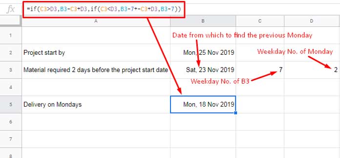
Formula in Cell B5: Calculating the Previous Monday
=IF(C3>D3, B3-C3+D3,
   IF(C3<D3, B3-7-C3+D3,
      B3-7
   )
)
The formula in cell B5 is not the final iteration. We’ll replace references to the helper cells C3 and D3 later.
This formula dynamically calculates the last occurrence of the specified previous day, i.e., Monday, based on the weekday number in cell D3.
Recap Illustration:
IF + WEEKDAY Combo Formula Explanation (Including Logic)
Let’s delve into how the formula calculates and identifies a specific previous day, specifically Monday, from the date in cell B3.
The formula encompasses two logical steps, each serving as a test:
Step 1 (Logical Test 1):
IF(WEEKDAY(B3)>2, B3-WEEKDAY(B3)+2This step examines whether the weekday number of the date in cell B3 is greater than 2 (representing Monday). If the result is TRUE, the formula executes B3-WEEKDAY(B3)+2 to ascertain the previous Monday.
Step 2 (Logical Test 2): If Step 1 Evaluates to FALSE
IF(WEEKDAY(B3)<2, B3-7-WEEKDAY(B3)+2To illustrate, let’s modify the date in cell B2 to 26/11/2019, consequently changing B3’s date to 24/11/2019.
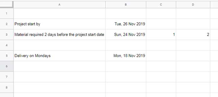
Here, the weekday of B3 is Sunday with a weekday number of 1 (as indicated in C3), executing B3-WEEKDAY(B3)+2 (Step 1) would only yield the next Monday. To correct this, we first deduct 7 days (one week) from B3 and that is B3-7-WEEKDAY(B3)+2.
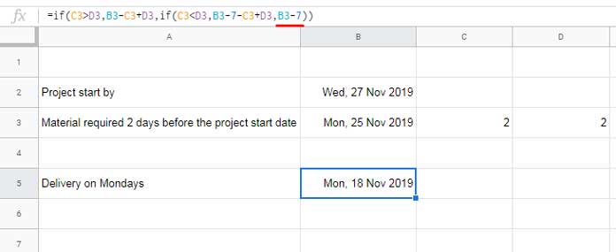
Step 3 (If Step 2 is FALSE):
B3-7Assuming the weekday numbers of the date in B3 and the specified day (Monday) are identical (as reflected in C3 and D3), you have the option, as per your preference, to either return B3 as is or deduct 7 days. In this formula, I’ve chosen the latter—B3-7.
Final Formula to Find the Previous Monday from a Date Input:
=IF(WEEKDAY(B3)>2, B3-WEEKDAY(B3)+2,
   IF(WEEKDAY(B3)<2, B3-7-WEEKDAY(B3)+2,
      B3-7
   )
)
To streamline the formula and prevent redundant calculations of WEEKDAY(), we utilized LET. This marks the conclusion of our final formula.
That wraps up the process of finding a specific previous day from a given date in Google Sheets.
Excellent, this saved me from banging my head against the wall for an hour or so. Anyway, my need was to determine the last Monday from the current date, so I did not refer to a specific cell and used the TODAY() function instead. I got it working by substituting all 7 references to cell B3 with TODAY() and thought perhaps I could call the TODAY() function only once using the LET() function. This is what I came up with:
=let(todaysdate, TODAY(), if(weekday(todaysdate)>2,todaysdate-weekday(todaysdate)+2,if(weekday(todaysdate)<2,todaysdate-7-weekday(todaysdate)+2,todaysdate-7)))I would recommend not using LET to avoid repeated references. The main purpose of LET is to prevent unnecessary calculations, so it’s advisable to define the WEEKDAY() calculation and then use that name in subsequent formula expressions.
In my tutorial, I have updated the formula accordingly. As a side note, it’s worth mentioning that LET was not available at the time of writing this post.