


")


")

")
")
 in Excel & Google Sheets")


When VLOOKUP returns multiple values using an array index, it often includes blanks or unwanted data. Filtering VLOOKUP result columns in Google Sheets helps you clean up the results and focus only on the values you need.
It helps you:
- Skip over blank cells
- Hide values you don’t need
- Or even apply conditions like “only show active employees” or “salary above 60,000.”
There are different ways to do this. Let’s go through them one by one with examples.
Example 1: Filter Out Blanks from VLOOKUP Result Columns
To start, we need to know how to return multiple columns using VLOOKUP. I’ve already explained that here: Retrieve Multiple Values Using VLOOKUP in Google Sheets.
Let’s walk through an example.
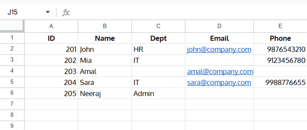
Sample Data
Formula
Suppose we want details for employee ID 202.
=ArrayFormula(VLOOKUP(202, A2:E, {2, 3, 4, 5}, FALSE))This searches for ID 202 in the first column of A2:E and returns the Name, Dept, Email, and Phone.
Result:
| Mia | IT | 9123456780 |
As you can see, the Email field is empty.
Filter Blanks with TOROW
To clean that up, wrap the formula with the TOROW function:
=ArrayFormula(TOROW(VLOOKUP(202, A2:E, {2, 3, 4, 5}, FALSE), 1))New Result:
| Mia | IT | 9123456780 |
Much better — the empty Email column is now gone.
Advanced Tip: What if you want to remove blanks not just from one lookup row but across multiple rows? The above approach won’t work. Instead, you can use BYROW with a LAMBDA helper.
For example, if your search keys are 201 and 203 in G2:G3, use:
You can use the following formula:
=BYROW(
  ArrayFormula(VLOOKUP(G2:G3, A2:E, {2, 3, 4, 5}, FALSE)),
  LAMBDA(row, FILTER(row, row<>""))
)
Result:
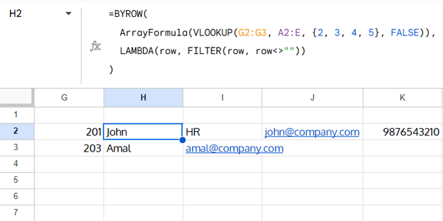
👉 Here’s what happens: BYROW processes each lookup row individually, while the LAMBDA tells it to remove blanks from that row.
This way, each row gets cleaned automatically. This approach is a bit more advanced, but it’s useful when working with multiple rows.
Example 2: Apply Conditions to VLOOKUP Results
Now let’s look at a different use case — filtering results based on conditions.
Sample Data
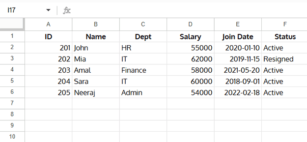
Say you want to look up multiple IDs, but only show them if their Status is Active.
Step 1: Regular VLOOKUP for Multiple IDs
IDs 201 and 202 in G2:G3:
=ArrayFormula(VLOOKUP(G2:G3, A2:F, {2, 3, 4, 5}, FALSE))Result:
| John | HR | 55000 | 2020-01-10 |
| Mia | IT | 62000 | 2019-11-15 |
Note: In some cases, the dates may appear as serial numbers instead of proper dates. If that happens, simply select the affected cells and apply Format > Number > Date to restore them to the correct date format.
Step 2: Filter VLOOKUP Results by Active Status (instead of just “Filter by Active”)
Instead of filtering the source range (which can throw #N/A), it’s cleaner to filter the VLOOKUP result itself:
=LET(
  vl, ArrayFormula(VLOOKUP(G2:G3, A2:F, {2, 3, 4, 5, 6}, FALSE)),
  FILTER(CHOOSECOLS(vl, 1, 2, 3, 4), CHOOSECOLS(vl, 5)="Active")
)
This formula first stores the VLOOKUP result in a variable vl.
ArrayFormula(VLOOKUP(G2:G3, A2:F, {2, 3, 4, 5, 6}, FALSE))→ looks up the IDs inG2:G3and returns Name, Dept, Salary, Join Date, and Status.CHOOSECOLS(vl, 1, 2, 3, 4)→ selects only the first four columns (ignoring Status).CHOOSECOLS(vl, 5)="Active"→ checks if the Status column equals “Active”.FILTER(..., ...)→ keeps only the rows where Status = Active.
So in short, this formula returns only Active employees’ details (Name, Dept, Salary, and Join Date) for the given IDs.
Step 3: Filter VLOOKUP Results by Salary Greater Than 60,000 (instead of just “Filter by Salary > 60,000”)
Same idea, different condition:
=LET(
  vl, ArrayFormula(VLOOKUP(G2:G3, A2:F, {2, 3, 4, 5}, FALSE)),
  FILTER(CHOOSECOLS(vl, 1, 2, 3, 4), CHOOSECOLS(vl, 3)>60000)
)
Now you’ll only see employees earning more than 60,000.
Wrapping Up
The trick is simple:
- Use TOROW if you just want to remove blanks.
- Use BYROW + LAMBDA to remove blanks across multiple rows.
- Use LET + FILTER + CHOOSECOLS if you want more advanced filtering, like conditions or comparisons.
Once you know these, VLOOKUP in Google Sheets becomes a lot more flexible.
Related Reading
- VLOOKUP with Multiple Criteria in Google Sheets: The Proper Way
- VLOOKUP Plus Next N Rows in Google Sheets – Return Multiple Rows
- Using VLOOKUP to Sum Multiple Rows in Google Sheets
- VLOOKUP to Search Across Multiple Columns in Google Sheets
- Excel VLOOKUP with Multiple Criteria and 2D Results (Dynamic Array)