


I am sure in this post you can learn something new! Let me clarify what I have included in this post, titled Filter values between two group headers in Google Sheets, first.
It’s like offset based on a dynamic group header/title value. Want a real-life example?
Sometimes you may not be able to filter a group of data if the data is not properly recorded like in a database.
For example, here is one table.
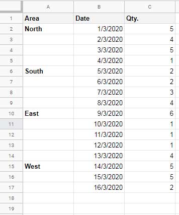
In this sample, the groups are the values “North”, “South”, “East”, and “West”. Can I filter the group “South”, I mean the rows 6 to 9?
Yes! It’s possible in two scenarios.
- If we know the row numbers, we can filter the group. See that here – Row Numbers as Filter Criteria in Google Sheets – How-To.
- The other option is filling the blank cells with the group headers using a formula – How to Repeat Group Labels for Filtering in Sheets.
But I want to do it dynamically. I mean I want to filter the values between the two group headers “South” and “East” without specifying the row numbers or repeating the group headers/titles.
How to Filter Values Between Two Group Headers in Google Sheets
In Google Sheets, we can dynamically filter rows between two strings (group headers). As a side note, the group headers can be numbers, strings, dates or any other special type characters.
You just need to specify the two values (group headers/titles) from a column. My formula will identify the rows and filter the correct range.
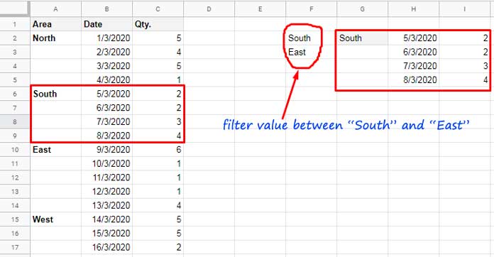
See the above image. I have specified two group header values in cell F2 and F3 to facilitate the filtering of one group “South”.
If I only specify a value in cell F2 and leave the cell F3 blank, then the formula, that you will get later, will populate all the rows from that group header.
To filter values between two group headers in a column I am going to use two key functions. They are Match and Indirect.
Let me write the formula from scratch so that you will be able to understand it.
Search Two Values in a Column and Form a Range Reference Using MATCH
Find Starting Row Number of a Group
As per my sample, column A is the column that contains the group header. If your column is different you may use the formula in that column.
We want to filter values between two group headers in Google Sheets. In that, the first group header is “South” which is in cell F2.
First, we will search the first group header which is “South” and find its row number (not relative position).
=MATCH(F2,$A:$A,0)Note: The search key is in column A. See I have used an entirely open range $A:$A in the formula. This open range is very important. Otherwise, you will end up getting the relative position of the search key in the match.
Result: 6
So the range to start the filtering is from cell A6. We can combine the letter “A” with the above number. It will be;
Formula_1:
="A"&MATCH(F2,$A:$A,0)Result: A6
Find Ending Row Number of a Group
Can we use the same above formula and only change the criteria which is the group name in F3 to get the ending row number of a group?
Nope!
=MATCH(F3,$A:$A,0)This formula will return the row number 10 which is the starting row number of the next group “East”. So we must use the below formula.
=MATCH(F3,$A:$A,0)-1Result: 9
We have to filter 3 columns. So here add the string “C” with the above result as below.
Formula_2:
="C"&MATCH(F3,$A:$A,0)-1Result: C9
We have two cell references generated dynamically and they are A6 and C9. We can make it a range by joining a colon in-between.
Generic Formula
=formula_1&":"&Formula_2In our case the formula is;
="A"&MATCH(F2,$A:$A,0)&":"&"C"&MATCH(F3,$A:$A,0)-1Result: A6:C9
Formula to Filter Values Between Two Group Headers in Google Sheets
We have now the range to filter rows between two group headers. That is the range A6:C9.
To populate this range simply wrap this formula with INDIRECT.
=INDIRECT("A"&MATCH(F2,$A:$A,0)&":"&"C"&MATCH(F3,$A:$A,0)-1)We are not yet completed! We must fine-tune the second MATCH used in this formula. Do you know, why?
Sometimes we need to filter all the rows below a group. In that case, we only specify one search string in cell F2. Then the cell F3 will be blank. This will cause an #N/A! error in the second Match.
So the second Match must be within IFNA as below.
=IFNA(formula_2,"")The purpose is like this. If the result of the ‘formula_2’ is #N/A! due to blank in F3, return a blank.
Modified Formula_2:
=ifna(MATCH(F3,$A:$A,0)-1,"")Here is the final formula to filter values between two group headers (titles) in Google Sheets.
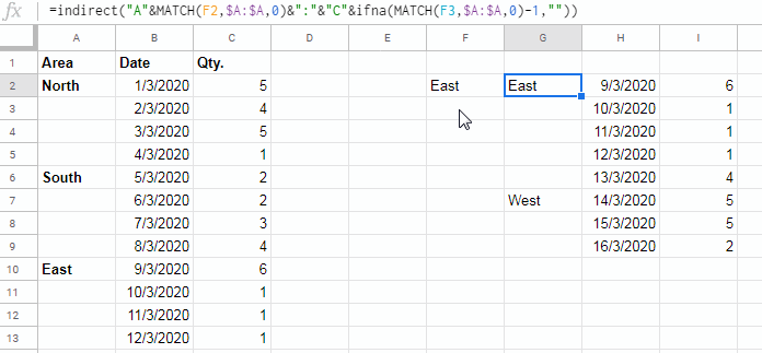
=indirect("A"&MATCH(F2,$A:$A,0)&":"&"C"&ifna(MATCH(F3,$A:$A,0)-1,""))The below live screenshot shows how the dynamic range formed using the Match and Indirect formulas filter a group.
Related Reading
- Filter Out Matching Keywords in Google Sheets – Partial or Full Match.
- Filter Groups Which Match at Least One Condition in Google Sheets.
- Alternating Colors for Groups and Filter Issue in Google Sheets.
- Formula to Conditionally Filter Last N Rows in Google Sheets.
- Get Total Only When Group | Subgroup Is Collapsed in Google Sheets.
- Google Sheets – Highlight the Max Value in Each Group.
- Vlookup Last Record in Each Group in Google Sheets.
- Extract First n Rows From Each Group in Google Sheets.
- Grouping and Subtotal in Google Sheets and Excel.
- Vlookup to Find Nth Occurrence in Google Sheets [Dynamic Lookup].