


")


")

")
")
 in Excel & Google Sheets")


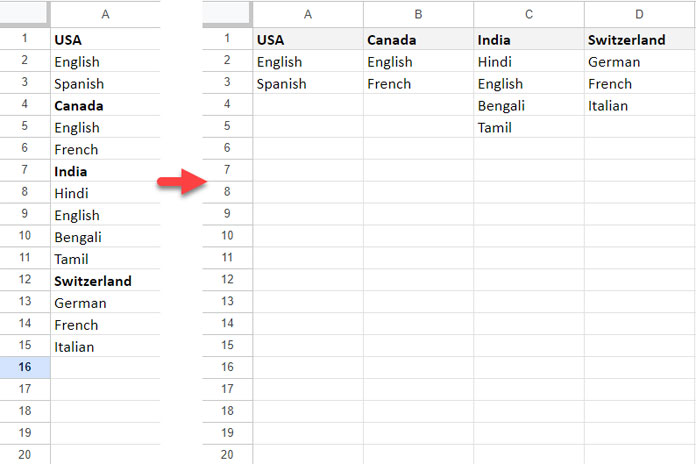
You may have data in several rows within a column, separated by headings. How do you extract the values between each heading into separate columns? Is that possible in Google Sheets?
Yes, you can filter or extract values between two headings using a range reference formed by two XLOOKUP functions in Google Sheets. If you have multiple headings, you can use the MAP function to iterate over an array of headings and separate the values into columns.
I’ll be sharing this relatively unknown technique with my readers.
To extract the values between two headings, you can use the following formula:
=XLOOKUP(heading1, range, range):XLOOKUP(heading2, range, range)Where:
heading1: The top heading.heading2: The bottom heading.range: The column ranges from which to extract data.
This result will include the two headers. You may need to use the FILTER function to remove those headers and any blank cells.
Example
Assume you have the following sample data in column A on Sheet1 of your Google Sheets file:
| A |
| USA |
| English |
| Spanish |
| Canada |
| English |
| French |
| India |
| Hindi |
| English |
| Bengali |
| Tamil |
| Switzerland |
| German |
| French |
| Italian |
In Sheet2 of the file, enter “USA” in cell A1 and “Canada” in cell B1.
How do you filter the data between the country names “USA” and “Canada” to get the key languages spoken in the USA?
Step 1: Extracting Values Between Two Headings, Including Headings
To extract the data between the headers ‘USA’ and ‘Canada’ in column A on Sheet1, enter the following formula in cell A2 on Sheet2:
=XLOOKUP(A1, Sheet1!$A$1:$A, Sheet1!$A$1:$A):XLOOKUP(B1, Sheet1!$A$1:$A, Sheet1!$A$1:$A)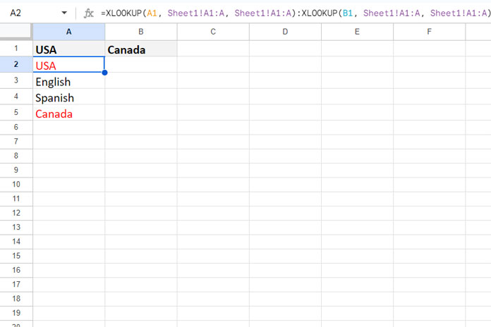
Note that this formula will include both headers. How can we remove them?
Step 2: Removing the Headings
Logic: Use the LET function to assign a name to the range formed by the XLOOKUP formulas and filter out the headers.
Enter the following formula in cell A2 on Sheet2:
=LET(data, XLOOKUP(A1, Sheet1!$A$1:$A, Sheet1!$A$1:$A):XLOOKUP(B1, Sheet1!$A$1:$A, Sheet1!$A$1:$A), FILTER(data, data<>A1, data<>B1, data<>""))The LET function assigns the name ‘data’ to the range reference created by the XLOOKUPs, and the FILTER function removes the headers and any blank rows.
Move Values Between Headings in a Column to Separate Columns
In the first row of Sheet2, enter the headings. Based on our sample data, enter the country names in cells A1:D1.
| A | B | C | D |
| USA | Canada | India | Switzerland |
Please enter the above formula in cell A2 and drag it across to D2.
The formula will return #N/A in D2 because it’s trying to get data between the header in D1 and the header in E1, which is blank.
| A | B | C | D |
| USA | Canada | India | Switzerland |
| English | English | Hindi | #N/A |
| Spanish | French | English | |
| Bengali | |||
| Tamil |
In cell E1, enter any character, for example, a hyphen (-).
Go to Sheet1 and enter a hyphen (-) in the first empty cell below the data in column A, such as A16. Now, check column D on Sheet2.
If you prefer using an array formula to move values between headings in a column to separate columns, clear all values in A2:D and enter the following formula in cell A2:
=MAP(A1:D1, B1:E1, LAMBDA(x, y, LET(data, XLOOKUP(x, Sheet1!A1:A, Sheet1!A1:A):XLOOKUP(y, Sheet1!A1:A, Sheet1!A1:A), FILTER(data, data<>x, data<>y, data<>""))))Explanation
The MAP function uses two arrays:
- Array 1:
A1:D1(Sheet2), which represents the range from the first header to the last header. - Array 2:
B1:E1(Sheet2), which represents the range from the second header to the last header plus one additional cell.
The LAMBDA function assigns names x and y to the values in these arrays. These names are used within the XLOOKUP functions to extract data between the headers specified by x and y.
The MAP function iterates through each pair of elements from these arrays (x and y) and returns the data that falls between the corresponding headers.
Resources
- Slicing Data with XLOOKUP in Google Sheets
- Lookup Header and Filter Non-Blanks in that Column in Google Sheets
- How to Move Values in Every Alternate Row to Columns in Google Sheets
- How to Move Each Set of Rows to Columns in Google Sheets
- Move Single Column to Multiple Columns Using Hlookup in Google Sheets
- Split Your Google Sheets Data into Category-Specific Tables