


")


")

")
")
 in Excel & Google Sheets")


Want to find out who appears most often in your data—like your top buyers, most frequent participants, or repeated responses? In Google Sheets, you can count how often each value appears in a list and easily filter the most frequent ones.
Whether you’re analyzing customer names, survey responses, or event attendance, this guide will show you a simple way to count and filter the most frequent strings in Google Sheets using built-in formulas—no manual work required.
Sample Data
| Event | Participant |
|---|---|
| Marketing Summit | Savannah |
| Dev Conference | Vincent |
| Marketing Summit | Savannah |
| Sales Workshop | Sandra |
| Dev Conference | Savannah |
| Sales Workshop | David |
| Dev Conference | Sandra |
| Marketing Summit | Vincent |
| Sales Workshop | Savannah |
| Dev Conference | Savannah |
Assume you have event data like this, with event names in column A and participant names in column B.
To find the top 3 participants who appear most frequently in the data, you can use the formula below.
Formula to Count and Filter Most Frequent Strings in Google Sheets
=SORTN(
   HSTACK(
      TOCOL(UNIQUE(range), 3),
      COUNTIF(range, TOCOL(UNIQUE(range), 3))
   ), n, 0, 2, FALSE
)- Replace
'range'with the range you want to analyze (e.g.,B2:Bto count participants). 'n'determines the number of top values to return (e.g.,3for the top 3).
Example
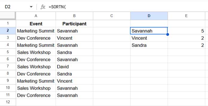
In the above example, to count and filter the most frequent 3 participant names, use the following formula:
=SORTN(
   HSTACK(
      TOCOL(UNIQUE(B2:B), 3),
      COUNTIF(B2:B, TOCOL(UNIQUE(B2:B), 3))
   ), 3, 0, 2, FALSE
)
Result:
Note: If you want to filter the top N most frequent strings plus any additional strings tied at the Nth position, replace the display_ties_mode value 0 in the SORTN function with 1.
For example, SORTN(…, 3, 1, 2, FALSE) will include all values that share the same count as the 3rd most frequent string.
How the Formula Filters Most Frequent Strings
The formula works in two simple steps:
- Get unique values and their counts:
HSTACK(
   TOCOL(UNIQUE(B2:B), 3),
   COUNTIF(B2:B, TOCOL(UNIQUE(B2:B), 3))
)UNIQUE(B2:B)extracts distinct strings from column B.TOCOL(..., 3)ensures the unique values are arranged vertically, skipping any empty cells.COUNTIF(B2:B, ...)counts how often each unique value appears.HSTACK(...)combines the values and their counts into a two-column array.
- Sort by count and return the top N results:
SORT(..., 3, 0, 2, FALSE)- SORTN selects the top 3 rows.
- The
2refers to the second column (count), which is used for sorting. - The
FALSEindicates descending order, showing the most frequent values first.
Additional Tip: Get Associated Values for the Most Frequent Strings
What if you want to filter the most frequent values in one column and extract associated values from another?
For example, the most frequent three participants from the sample data are:
- Savannah
- Vincent
- Sandra
To get the associated events for each of these names, use this two-step setup:
Step 1: Get Top Participants (in D2)
=CHOOSECOLS(
   SORTN(
      HSTACK(
         TOCOL(UNIQUE(B2:B), 3),
         COUNTIF(B2:B, TOCOL(UNIQUE(B2:B), 3))
      ), 3, 0, 2, FALSE
   ), 1
)
Used CHOOSECOLS to return only the first column (the values), excluding the count column.
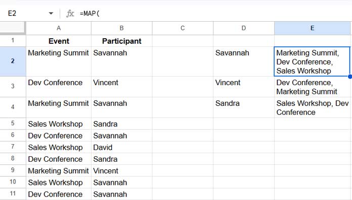
Step 2: Get Their Associated Events (in E2)
=MAP(
   D2:D,
   LAMBDA(
      row,
      TEXTJOIN(", ", TRUE, UNIQUE(FILTER(A2:A, B2:B=row)))
   )
)
This will return a comma-separated list of events attended by each top participant.
Resources
- How to Use Google Sheets MODE (MODE.SNGL) Function
- How to Use the MODE.MULT Function in Google Sheets
- Get the Mode of Text Values in Google Sheets
- How to Find Mode of Comma-Separated Numbers in Google Sheets
- Mode of Comma-Separated Numbers in Excel (Dynamic Array)
- Get Most Frequent Keywords from Titles in Google Sheets
- Finding Most Frequent Text in Excel with Dynamic Array Formulas