Google Sheets: Show Only the Last Status Change per Name

When managing employee records or project updates in Google Sheets, it’s common to have multiple rows for the same person across different dates. However, in many cases, you only need the last status change per name—the most recent entry that reflects their current role or position.

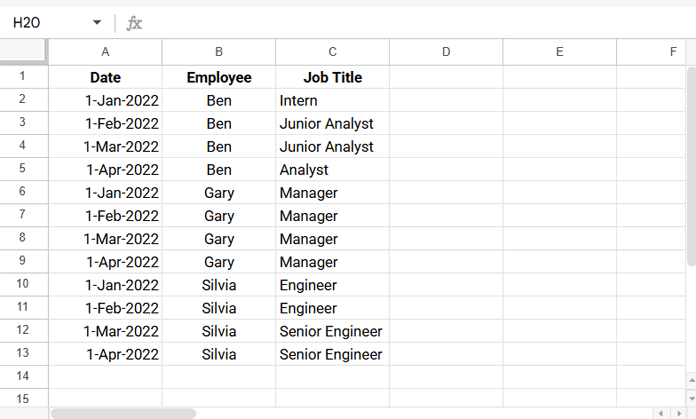
For example, Silvia was added as an Engineer on Jan 1, 2022, stayed in the same role on Feb 1, 2022, and was promoted to Senior Engineer on Mar 1, 2022. She also appears in the following months, but since her role didn’t change after Mar 1, the last status change row in Google Sheets is the record of Mar 1, 2022.

In this tutorial, you’ll learn step by step how to filter the last status change rows in Google Sheets so your dataset shows only the latest updates for each person. This makes your sheet cleaner, easier to read, and more useful for reporting.

Table of Contents

Sample Data

Here’s a sample dataset in A1:C:

Sample employee status data in Google Sheets showing multiple rows per person with job title changes across different dates

Expected Output

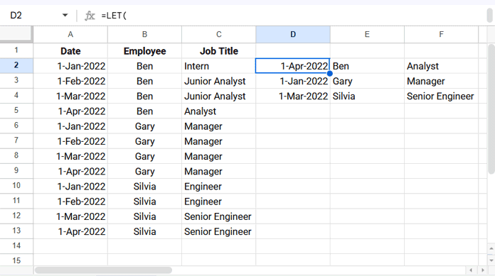
From this dataset, the last status change rows per employee should be:

Filtered data in Google Sheets showing only the last status change per employee

Why Not Use QUERY or FILTER?

The QUERY and FILTER functions are great for criteria-based filtering, but in this case, they can’t easily isolate only the last status change per name.

Instead, we’ll use a combination of SORT and SORTN to achieve this.

(Note: The formula works even if your data isn’t sorted, but keeping it sorted by date makes it easier to cross-check the results manually.)

How to Show Only the Last Status Change per Name in Google Sheets (Formula)

Here’s the formula you can use (assuming your data is in A2:C). Enter it in D2:

=LET(  
  srt, SORT(A2:C, 1, TRUE),  
  uniq, SORTN(srt, 9^9, 2, 2, TRUE, 3, TRUE),  
  SORTN(SORT(uniq, 1, FALSE), 9^9, 2, 2, TRUE)  
)

Make sure there’s enough empty space below and to the right of the formula cell for the results to spill.

Step-by-Step Formula Explanation

This formula works in three steps:

Step 1: Sort the Data by Date

SORT(A2:C, 1, TRUE)

Sorts the dataset by the Date column, so the latest entries appear at the bottom.

Step 2: Extract Unique Employee and Job Title Combinations

SORTN(srt, 9^9, 2, 2, TRUE, 3, TRUE)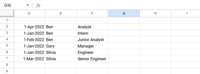

Applying SORTN in Google Sheets to extract unique employee and job title combinations while keeping dates

UNIQUE(B2:C) would give you only the distinct Employee + Job Title pairs, but it drops the Date column, which we need. Instead, we run SORTN on the full 3-column range (srt) so that the Date stays attached to each returned row.

9^9 is just a very large n so all rows are considered.
The 2 argument (display-ties mode) together with the following column arguments tells SORTN to return one row per unique combination of the columns we care about (here Employee = column 2 and Job Title = column 3).
Because srt was sorted by Date ascending (oldest → newest), this SORTN call keeps the first occurrence of each Employee+JobTitle pair — i.e., the date when that title first appeared for that employee.

Step 3: Return the Last Status Change per Employee

SORTN(SORT(uniq, 1, FALSE), 9^9, 2, 2, TRUE)

First, sorts the unique dataset by Date (descending).
Then removes duplicates by Employee (column 2).
The result is the latest status change row for each person.

Additional Tip: Handling Cases Where a Previous Status Reappears

The formula we discussed above works for most cases, but there’s a scenario it won’t handle correctly: if an employee’s previous status resurfaces later.

For example:

An employee joins as Engineer, gets promoted to Senior Engineer, and later is demoted back to Engineer.
Using the SORT + SORTN formula we discussed earlier, the last status change row would incorrectly return the Senior Engineer entry, because it only considers the first occurrence of each Employee + Job Title combination in the sorted data.

To handle this scenario, you can use a different approach. Important: your data must be sorted first by Date, then by Employee. Here’s the formula:

=UNIQUE(
  MAP(B2:B, LAMBDA(val, 
    ARRAYFORMULA(XLOOKUP(val&XLOOKUP(val, B2:B, C2:C, , 0, -1), B2:B&C2:C, A2:C)))
  )
)

How It Works:

Inner XLOOKUP searches from bottom to top to find the latest status of each employee.
Outer XLOOKUP searches from top to bottom for that status and returns the row corresponding to the last status change.
MAP applies this logic to each employee individually, and UNIQUE ensures only the distinct last status change rows are returned.

This approach ensures that even if a previous status reappears later, the formula correctly identifies the latest change per employee.

Final Thoughts on Filtering Last Status Change Rows

By combining SORT and SORTN, you can efficiently filter out only the last status change per name in Google Sheets for most typical cases. This method is flexible, works even if your data isn’t perfectly sorted, and helps keep your reports concise and accurate.

For scenarios where an employee’s previous status resurfaces later, the alternative XLOOKUP + MAP formula can handle these edge cases, ensuring that the latest status change is always captured.

Using these approaches together gives you a robust way to manage employee or project status data while keeping your Google Sheets clean and easy to analyze.

Copy Sample Sheet