This tutorial explains how to filter data for a specific number of past weeks in Google Sheets, such as 1 week, 2 weeks, 3 weeks, etc.

The formula provides complete control, allowing you to dynamically specify the number of weeks and also choose whether the week starts on Sunday or Monday.

If the current week is ongoing and it’s not yet the weekend, it will be excluded from the filter. If you wish to include it, the starting day of the week becomes irrelevant, making the process simpler.

I’ll demonstrate two options to filter data for a specific number of past weeks in Google Sheets:

1. Filter from today’s date to the past n weeks.
2. Filter the data from the past n full weeks.

Both of these can be achieved using either the Filter menu or the FILTER function, and I’ll explain both methods.

Sample Data Preparation

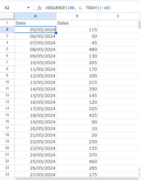
For this example, we’ll use sample data spread across two columns in Sheet1. The first column contains the Date and the second column contains Sales.

If you are learning the technique to filter data for a certain number of past weeks and don’t have sample data to test, you can create some sample data as follows:

Enter “Date” in cell A1 and “Sales” in cell B1.

Enter the following formula in cell A2 to generate a sequence of dates suitable for testing:

=SEQUENCE(100, 1, TODAY()-60)

This formula generates a sequence of dates starting from 60 days ago and fills 100 rows with these dates.

In cells B2:B101, enter some random numbers to use as sales amounts.

Alternatively, you can enter this formula in cell B2 to generate a sequence of numbers.

=SEQUENCE(100)

Your sample data is now ready for testing!

Filter Data for a Specific Number of Past Weeks from Today’s Date

Which method do you prefer? Using the FILTER function or the Data Menu Filter command?

Let’s explore both methods, starting with the formula.

Using the FILTER Function

The sample data is in Sheet1. In another sheet in the same file, enter the following formula in cell A2:

=FILTER(Sheet1!A2:B, Sheet1!A2:A >= TODAY()-1*7)

Where:

• Sheet1!A2:B is the range to filter, excluding the header row.
• Sheet1!A2:A >= TODAY()- 1*7 is the condition to filter where Sheet1!A2:A is the date range, excluding the header row.

This formula filters data from the past week onwards. To get data from the past two weeks, replace 1*7 with 2*7.

If you want to exclude future weeks from your filter range, use an additional condition. The formula will be as follows:

=FILTER(Sheet1!A2:B, Sheet1!A2:A >= TODAY()-1*7, Sheet1!A2:A < TODAY())

Using the Filter Menu

If you prefer the filter menu, follow these steps:

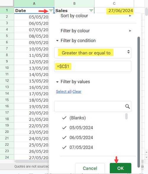
1. Enter =TODAY() - 1*7 in an empty cell in Sheet1, preferably in cell C1.
2. Select your data range.
3. Click Data > Create a filter.
4. Click on the filter icon in cell A1.
5. Select Filter by condition.
6. Choose Greater than or equal to and enter =$C$1 in the given field.
7. Click OK.

This formula filters the dates in column A to show only those dates that are within the last 1 week (7 days).

To filter data for the past 4 weeks, replace 1 in the formula in cell C1 with 4. Then click the filter drop-down in cell A1 and click OK.

This will also include future dates if they are present. To filter out future dates, follow these steps:

1. In cell D1, enter =TODAY() - 1.
2. Within the Filter drop-down menu, select Is between instead of Greater than or equal to.
3. Enter =$C$1 in the first field and =$D$1 in the second field.

Filter Data for the Past N Full Weeks in Google Sheets

Unlike the previous formula, here we need to consider important aspects such as whether the week starts on Sunday or Monday and that today is in the middle of the current week.

This formula might be a little complex but is manageable since I used the LET function to simplify reading the formula and improve performance.

Formula:

=LET(
   range, Sheet1!A2:B, n, 1, wds, "Sunday", 
   ws, TODAY()-WEEKDAY(TODAY(), SWITCH(wds, "Sunday", 1, "Monday", 2)), 
   FILTER(range, Sheet1!A2:A>ws-(n*7), Sheet1!A2:A<=ws)
)

Enter this formula in cell A2 in another empty sheet in the same file.

Explanation:

• range is the range to filter (A2:B).
• n is the number of past full weeks to filter (1 in this example).
• wds is the name of the week start day, where you can specify either ‘Sunday’ or ‘Monday’.
• ws is the previous week’s end date calculated as:
  TODAY()-WEEKDAY(TODAY(), SWITCH(wds, "Sunday", 1, "Monday", 2)), which returns the previous week’s end date. Essentially, this is TODAY() - WEEKDAY(TODAY(), 1).
  In the formula, I have replaced 1 in WEEKDAY(TODAY(), 1) with SWITCH(wds, "Sunday", 1, "Monday", 2) to return the weekday number dynamically.

Formula Explanation:

FILTER(range, Sheet1!A2:A > ws - (n * 7), Sheet1!A2:A <= ws)

The FILTER function filters the date range between ws - (n * 7) (exclusive) and ws (inclusive).

Can I Use the Filter Menu to Filter Data for the Past N Full Weeks?

Yes. In the above formula, you need to make a minor change to get the date range to filter.

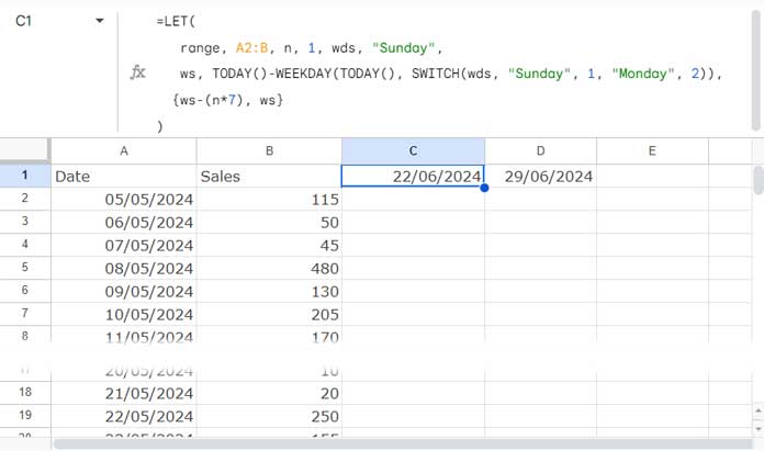
Replace FILTER(range, Sheet1!A2:A > ws - (n * 7), Sheet1!A2:A <= ws) with {ws-(n*7), ws} and enter it in cell C1 in Sheet1. This will return the start and end date range in C1:D1.

=LET(
   range, A2:B, n, 1, wds, "Sunday", 
   ws, TODAY()-WEEKDAY(TODAY(), SWITCH(wds, "Sunday", 1, "Monday", 2)), 
   {ws-(n*7), ws}
)

Select A1:B and click Data > Create a filter.

In the filter drop-down in cell A1, click Filter by condition and select Is between.
Enter =$C$1 and =$D$1 in the respective fields and click OK.

This will filter the data for the last 1 week. If you want to filter the data for the last 2 weeks, replace n, which is 1 in the formula, with 2.

Then don’t forget to click the A1 filter drop-down and click OK to apply the changes.

Resources

• Filter Data Based on This Week, Last Week, Last 30 Days in Google Sheets
• Filter or Find the Current Week This Year and Last Year in Google Sheets
• How to Filter Current Week Horizontally in Google Sheets
• Finding Week Start and End Dates in Google Sheets: Formulas
• Calculate Week Number Within Month (1-5) in Google Sheets
• Find the Date or Date Range from Week Number in Google Sheets
• Weekday Name to Weekday Number in Google Sheets
• Reset Week Number in Google Sheets Using Array or Non-Array Formulas
• Same Day Last Week Comparison in Google Sheets
• Insert Blank Rows to Separate Week Starts/Ends in Google Sheets
• Convert Dates to Week Ranges in Google Sheets (Array Formula)