To fill zero values in blank cells, you can use either the Find and Replace command or a formula in Google Sheets.

Find and Replace command:

This method is suitable for filling zero in blank cells in a data range that doesn’t contain formulas.

The reason for its suitability lies in how it handles formulas:

If a formula in the range returns a single value (non-array formula) and that value is blank, this approach will replace that formula with zero. However, if a formula in the range returns multiple values (array formula) and any of the values are blank, the formula will replace that cell with zero, potentially breaking the formula as it may not expand due to the newly filled value.

Formula Approach:

You can use it with existing formulas to replace blanks with zero, or apply a standalone formula to populate a new range with blank cells filled with zero.

It’s important to understand both options to effectively manage your data in Google Sheets.

Find and Replace to Fill Blank Cells with Zeros

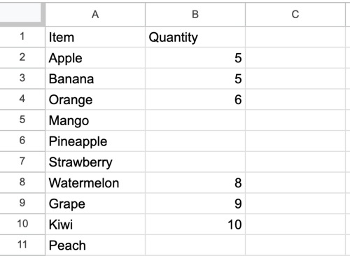
I have data in columns A and B (cell range A1:B11), and some cells in column B are blank. There are no formulas in use anywhere in this range.

Note: You can use a highlighting rule to easily find any cell in the range containing formulas. You can check out: How to Highlight All the Cells with Formulas in Google Sheets.

I want to fill those blank cells with the value zero while keeping the other values in that range intact.

Steps to Follow:

1. Format Cells as Plain Text and Revert to Automatic (Must Do):
   • Select the range where you want to fill blank cells with zeros, here B1:B11.
   • Click Format > Number > Plain Text. This will format the numbers as text.
   • While keeping the selection, click on Format > Number > Automatic to revert to the original formatting.
2. Find and Replace:
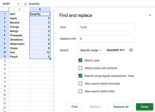
   • Select the range B1:B11 if not already selected.
   • Click Edit > Find and Replace (you can alternatively use the keyboard shortcut Ctrl + H in Windows or ⌘ + Shift + H in Mac).
   • In the Find field in the Find and Replace window, enter the following regular expression: ^\s*$
   • In the Replace with field, enter 0.
   • Tick “Search using regular expressions” and “Match case.”
   • Click Replace All.

This will fill all blank cells in B1:B11 with zeros while retaining other values in the range.

Formula Approach to Replace Blank Cells with Zeros

As mentioned, using Find and Replace might not be feasible in a complex data range containing formulas.

In such cases, you can use a formula with the drawback that it generates a new range with blank cells replaced with zero.

Generic Formula:

=ArrayFormula(LET(range, range_reference, IF(range="", 0, range)))

In this formula, replace range_reference with the range in which you want to replace blanks with zero values.

For example, in our previous scenario, you can use the following formula in cell C1:

=ArrayFormula(LET(range, B1:B11, IF(range="", 0, range)))

However, if you’re using an array formula such as a FILTER or QUERY that contains blank cells in their output, you can still follow the above generic formula. In that case, replace range_reference with the formula in question itself.

Resources

• Replace Blank Cells with 0 in Query Pivot in Google Sheets
• How to Fill Empty Cells with 0 in Pivot Table in Google Sheets
• Array Formula to Fill Blank Cells With the Values from Cell Above
• Fill Blank Cells with the Text Below in Google Sheets
• How to Highlight Blank Cells Using Value from Cell Above in Google Sheets
• How to Sort Rows to Bring the Blank Cells on Top in Google Sheets