


")


")

")
")
 in Excel & Google Sheets")


You can use a FILTER and COUNTIFS combo formula to extract the first N rows from each group in Google Sheets. Another option is using QUERY with COUNTIFS, but that approach tends to be more complex.
Extracting the first N rows from each group is useful in many scenarios, such as:
- Retrieving the first N customer orders for each product category.
- Getting the first N tasks assigned to each team or employee.
- Extracting the first N test scores for each student.
And so on.
Generic Formula
=SORT(FILTER(data, COUNTIFS(col, col, ROW(col), "<="&ROW(col))<=n), coln, TRUE)How to Use This Formula
Replace the placeholders as follows:
data: The data range to process (excluding the header row).col: The column that defines the group (e.g., date, category, or ID).n: The number of rows you want to extract from each group.coln: The column number ofcolwithindata.
Example: Extracting the First N Rows From Each Group
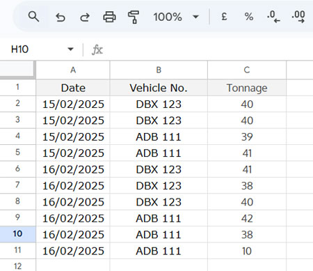
Consider the following trip log:
Extract the First 2 Trips for Each Day
=SORT(FILTER(A2:C, COUNTIFS(A2:A, A2:A, ROW(A2:A),"<="&ROW(A2:A))<=2), 1, TRUE)| Date | Vehicle No. | Tonnage |
| 15/02/2025 | DBX 123 | 40 |
| 15/02/2025 | DBX 123 | 40 |
| 16/02/2025 | DBX 123 | 41 |
| 16/02/2025 | DBX 123 | 38 |
Extract the First 2 Trips for Each Vehicle
=SORT(FILTER(A2:C, COUNTIFS(B2:B, B2:B, ROW(B2:B),"<="&ROW(B2:B))<=2), 2, TRUE)| Date | Vehicle No. | Tonnage |
| 15/02/2025 | ADB 111 | 39 |
| 15/02/2025 | ADB 111 | 41 |
| 15/02/2025 | DBX 123 | 40 |
| 15/02/2025 | DBX 123 | 40 |
Formula Explanation
The formula uses two key functions:
- FILTER: Extracts rows where the condition evaluates to TRUE.
- COUNTIFS: Creates a running count of occurrences for each group.
The condition:
COUNTIFS(B2:B, B2:B, ROW(B2:B), "<="&ROW(B2:B))<=2COUNTIFS(B2:B, B2:B, ROW(B2:B), "<="&ROW(B2:B)): Counts how many times each value appears up to the current row.- The condition
<=2ensures that only the first 2 occurrences per group are included in the result.
This method allows you to dynamically extract the first N rows from each group.
Bonus: Extracting the Last N Rows From Each Group
To extract the last N rows instead of the first, simply modify the condition:
Change:
"<="&ROW(A2:A)To:
">="&ROW(A2:A)
This is the best. Thank you!
I’ve first sorted my data by group, then by value. Would there be a way to return multiple rows if there was a tie for the largest value?
It’s fine if this requires helper columns, but I would like them to dynamically grow to fit the data. I greatly appreciate your help!
Hi, David,
That seems possible with SORTN Tie Modes.
Can you create your sample data and share the sheet with me. It won’t be published.
You can leave the sample sheet URL via reply below.
Prashanth,
Col5 is the Login Time Stamp, Col1 is the Username.
I need the resulting table to show the first Login Time Stamp per Username and all dates.
So, the list should show a unique Time Stamp (Minimum) per Username and Date.
I think this is like a “Group by Date,” but I have no idea how to do it.
Thanks, I appreciate any help on it!
Hi, Jose,
I’m not clear.
If you want to group data, there should be an aggregation column. Also, you must convert timestamp to date.
You can start with this.
=ArrayFormula(QUERY({A1:D,{"Date";INT(E2:E)},F1:H},"Select * where Col1 is not null"))Or share a sample sheet link below.
Hey, thanks a lot for this, it’s very useful!
Would you know how I can extract the top n% values from each group?
I have a column A which contains the Group names and B some score values, and for each group name I’d like to be able to select the top 10%
best scores.
Have a great day,
Lorraine
Hi, Lorraine,
I do have a solution that using non-array formula.
I will post it soon.
In the meantime, if you share an example sheet by leaving the URL in your reply, I may be able to use that as the base/source data to write the post.
Hi, Lorraine,
See if this tutorial helps?
How to Get the Top N Percent Scores From Each Group in Google Sheets.
Is there a way to get this to work on a different sheet/tab? I have 7 columns (A:G) and I’m able to get it to work on the same sheet/tab as my source data but not on a different one. I’m adding the name of the source data sheet but I’m getting errors. Thanks.
Hi, Jason,
If your sheet name contains space, you should include the single quote surrounding the sheet name.
Eg:
Sheet Name: product summary
Range: A2:B
It should be referred to in the formula as;
'product summary'!A2:Bnotproduct summary!A2:BIf this doesn’t help, share your sheet link in reply which won’t be published (remove personal/confidential info from the sheet).
Hey!
Thanks a lot for the trick!
What if I want to combine two tabs? they have the same structure.
Thanks.
Hi, Bob,
To combine values in columns A and B in ‘Sheet1’ and ‘Sheet2’, use this formula.
=Query({Sheet1!A:B;Sheet2!A:B},"Select * where Col1 is not null")On this output, you can use my formula to extract first ‘n’ rows.
Thanks
That for column A:B. What about I have columns A, B, C, D, and E?
=Query({sort(A2:E,1,0),ARRAYFORMULA(COUNTIFS(sort(A2:A,1,0),sort(A2:A,1,0),ROW(A2:A),"<="&ROW(A2:A)))},"Select Col1,Col2,Col3,Col4,Col5 where Col6<=2")