You can use COUNT or COUNTA with BYROW, or use MMULT and DCOUNT/DCOUNTA as alternative options to expand count results in Google Sheets.
The COUNT function (for numeric counts) and the COUNTA function (for counting all values) take an array and return a single-cell output.
For example, you can use them to count values in a row, but they do not provide row-by-row outputs, even when used with ARRAYFORMULA.
You can convert them into a custom LAMBDA function to use with BYROW for expansion, or choose MMULT, DCOUNT (for numeric values), or DCOUNTA (for all values). We will explore all these options.
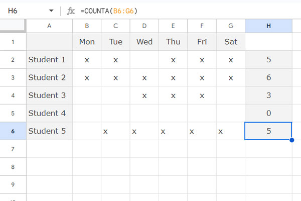
In this example, I have student names in column A and their weekly attendance in columns B to G. Specifically, the names are in A2:A6, and the attendance from Monday to Saturday is in B2:G6. A checkmark in the grid indicates a present student.

The following formula in cell H2 will return the count of values in B2:G2:
=COUNTA(B2:G2)Drag the fill handle from H2 down to H6 to get the count for each row.
How do you expand the count results from H2 down the column?
Expand Count Results with BYROW
In the above example, we used the following COUNTA formula in cell H2:
=COUNTA(B2:G2)You can turn it into an unnamed function using LAMBDA as follows:
LAMBDA(row, COUNTA(row))We can then use this in BYROW like this:
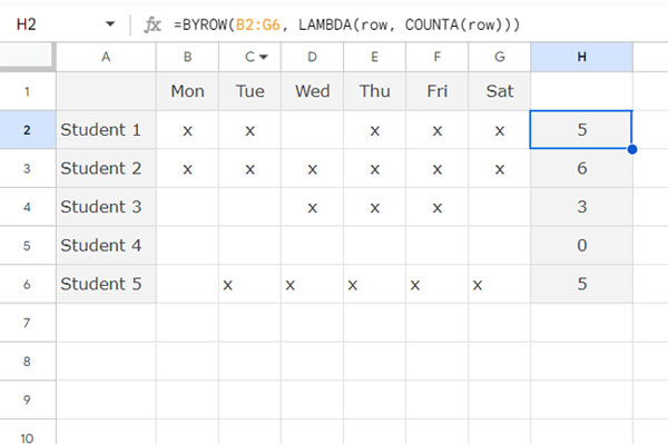
=BYROW(B2:G6, LAMBDA(row, COUNTA(row)))
The BYROW function applies the custom LAMBDA function to each row in the array B2:G6 and returns a row-wise count result.
You can replace COUNTA with COUNT if you want to count numeric values, such as numbers, dates, or times.
This is the easiest way to expand count results in Google Sheets. Let’s move on to the other two options.
Expand Count Results with Database Functions
Here, database functions refer to the DCOUNT and DCOUNTA functions.
Since we want to expand the count results of text values (check marks), we will use DCOUNTA.
You can use the following formula in cell H2 to expand the count results to H2:H6:
=ArrayFormula(
   TRANSPOSE(
      DCOUNTA(
         VSTACK(SEQUENCE(1, ROWS(B2:G6)), TRANSPOSE(B2:G6)),
         SEQUENCE(1,ROWS(B2:G6)),
         {IF(,,); IF(,,)}
      )
   )
)
If you need to count numeric values, simply replace DCOUNTA with DCOUNT in the above formula.
This formula is more complex compared to the BYROW formula but is still easy to understand.
Formula Explanation (DCOUNTA)
Syntax: DCOUNTA(database, field, criteria)
DCOUNTA can return the count of values in each column at once.
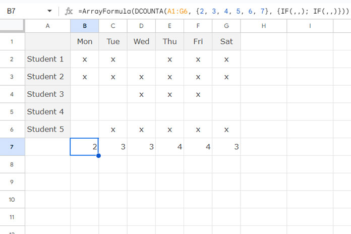
For example, the following formula in cell B7 can return the count of values in each column, with results in B7:G7:
=ArrayFormula(DCOUNTA(A1:G6, {2, 3, 4, 5, 6, 7}, {IF(,,); IF(,,)}))
Where A1:G6 is the database to count, {2, 3, 4, 5, 6, 7} are the columns (fields) to count, and {IF(,,); IF(,,)} is the criteria to count, which means counting all values.
However, DCOUNTA cannot expand vertically.
Therefore, we will transpose the range (change the orientation), count the columns, and then transpose the result.
In our H2 formula, here are the arguments in use:
- database:
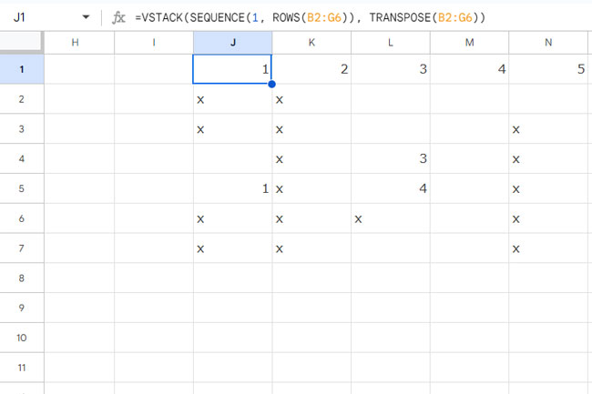
VSTACK(SEQUENCE(1, ROWS(B2:G6)), TRANSPOSE(B2:G6))TRANSPOSE(B2:G6)– This transposes the range B2:G6.SEQUENCE(1, ROWS(B2:G6))– This returns a row of sequence numbers matching the number of rows in the range.VSTACK(..., ...)– This appends the row numbers above the transposed range. This results in a transposed range with a header row, fulfilling the structured data requirement.
- field:
SEQUENCE(1, ROWS(B2:G6))– This dynamically returns the column numbers to total. - criteria:
{IF(,,); IF(,,)}– Empty criteria mean to count all values.
The DCOUNTA function will return the count of each column in the transposed data. By transposing the result, we obtain the expanded count results for each row.
Expand Count Results with MMULT
This method is simpler than using database functions.
Enter the following MMULT-based formula in cell H2 to expand the count results vertically in the range H2:H6:
=ArrayFormula(TRANSPOSE(
   MMULT(
      SEQUENCE(1, COLUMNS(B2:G6), 1, 0),
      TRANSPOSE(N(B2:G6<>""))
   )
))
This formula uses matrix multiplication to return expanded count results. Here’s how it works:
Formula Explanation (MMULT)
Syntax:
MMULT(matrix1, matrix2)Where:
- matrix1:
SEQUENCE(1, COLUMNS(B2:G6), 1, 0)
The SEQUENCE function generates numbers across the columns equal to those in range B2:G6. With a step of 0 and starting at 1, it creates an array like {1, 1, 1, 1, 1, 1}. - matrix2:
TRANSPOSE(N(B2:G6<>""))
This converts the range into an array of 1s (for non-empty cells) and 0s (for empty cells) and transposes it.
The number of columns in matrix1 (6) matches the number of rows in matrix2 (6), satisfying the conditions for matrix multiplication.
The MMULT function calculates the count for each column in the transposed range. After transposing the result, it provides the expanded counts vertically.
To get expanded count results for numeric values, replace matrix2 with:
TRANSPOSE(N(ISNUMBER(B2:G6)))This modification ensures that only numeric values are counted, as ISNUMBER checks whether each cell contains a number.
Resources
- Get the Count of Occurrences in Each Row in Google Sheets (Combo Formula)
- Count Blank Cells Row by Row in Google Sheets (COUNTBLANK Each Row)
- DCOUNT to Count Values in Each Column in a Table in Google Sheets
- Running Count in Google Sheets: Formula Examples
- Reverse Running Count Simplified in Google Sheets
- Fix Interchanged Names in Running Count in Google Sheets
- Case-Sensitive Running Count in Google Sheets
- Running Count of Occurrences in Excel (Includes Dynamic Array)


Hello,
Thank you for your help! I have a table with arrays that create details by row, and I want to count them. However, the count is simply seeing a value in every cell, so 5 is returned for all rows.
This is the formula I am using:
=BYROW(AY6:BC,LAMBDA(ROW,IF(COUNTA(row)=0,,COUNTA(row))))The range AY:BC usually has an expected count of 1 or 2 for each row, so I know that 5 is wrong.
Hi Charles Jackson,
I think you are using formulas in the range that returns an empty string, such as
"". You can replace""withIF(,,)in those formulas.For example, you can replace the formula
=IF(1=1,"",2)with the formula=IF(1=1,IF(,,),2).The
IF(,,)function will return a null string.Yes, I managed to figure that out later on and switched to a COUNTIF, although determining the correct point in my nesting was trial and error. lol
Many thanks Prashanth!
I have a spreadsheet with multiple rows, causing it to need an arrayformula for calculation, and I’m trying to take a count of the columns with the value of 5 for each row (separately).
I am confused on how do I change your original formula to only count the ones with a value of 5.
I keep getting formula errors.
Hi, Tyrtle,
In the above tutorial, find the side note just above the sub-title “Expanding Count Results in Google Sheets Using MMULT.”
In that tutorial, you can find a possible solution (sample sheet included in that tutorial)
Hi Prashanth,
I find your tutorials quite useful. Thanks.
I was looking for counting the occurrence of substrings in an array formula which brought me to this page. I did test your approach and work quite well. however, the problem I have is slightly different from the example you have on this page.
Basically, I have rows that include employee name, start & end dates, variable ranges of weekdays (from Monday through Sunday), and weekly work hours. I want to create a matrix that displays the 7 days of the week, daily hours for each day with a “None” for the missing days; please see below for an example:
StartDate|EndDate|WeeklyHours|Weekdays
02/05/20|30/05/20|16|Monday, Friday
03/03/20|31/03/20|28|Monday, Wednesday, Friday, Sunday
02/05/20|29/05/20|18|Monday, Thursday, Friday
I would like to add a column to the right calculating the average daily hours for each row. In the above case, it will be:
StartDate|EndDate|WeeklyHours|Weekdays|DailyHours
02/05/20|30/05/20|16|Monday, Friday|8
03/03/20|31/03/20|28|Monday, Wednesday, Friday, Sunday|7
02/05/20|29/05/20|18|Monday, Thursday, Friday|6
I did try your approach, step by step, and using the SPLIT function too (again, using your tutorial):
To create Matrix1, I used the following formula, which worked well:
=iferror(ArrayFormula(len(iferror(SPLIT(D2:D,",")))/len(iferror(SPLIT(D2:D,",")))),0)
To create Matrix2, I used the following formula, which failed with the error “Argument must be a range”:
ArrayFormula(Transpose(column(iferror(SPLIT(D2:D,","))))^0)I guess this fails because it is expecting physical columns, generated from Matrix1 calculation.
Any thoughts?
Your reply will be much appreciated.
Regards
Hi, Sabba,
For the range A1:D and the row A1:D1 contains headers, then use following MMULT in E1.
={"Average";ArrayFormula(if(len(A2:A),C2:C/mmult(if(iferror(split(D2:D,","))<>"",1,0),
transpose(sequence(1,columns(if(split(D2:D,",")<>"",1,0)))^0)),))}
This would return the average as per your requirement.
Thanks a lot. Worked like a charm!
Regards
Hi Prashanth,
I appreciated what you do!
for sure will come here again for your best guide.
Wish you a great ilfe!
Thank You.
This is so great!
Really appreciated, thank you Prashanth
For the best result, please help with the result from the formula in C2:D to be blank if equal or less then 0.
Hi, Bahar,
Already done! For other readers, who wish to know how to achieve the said result, please read this post.
Two Ways to Remove 0 Values in Google Sheets [How to]
MMULT Formula to Count Values in Each Row.
Hi, how if I want to count values >0 in each row? please help.
Thank You.
Hi, Bahar,
Change Matrix1 to;
=ArrayFormula(if(n(B2:G8)>0,1,0))The N function around the range B2:G8 helps to skip text strings. The IF function returns 1, if the value is greater than 1, else 0.
Hi Prashanth,
I appreciated what you do!
I hope you can help on this finishing, make it blank if 0?
Thank You.
Hi, Bahar,
You were asking me a formula to count the numbers greater than 0 in each row. I’ve provided the solution but the range (matrices) is as per my sample data.
If you want the formula as per your data, I may require access to your sheet (only demo data required).
Hi Prashanth,
Sure, here is the sheet 🙂 I appreciated what you do!
—Link removed – admin —
Thank You.
Hi, Bahar,
Seen your sheet and updated the formula. Actually you just need to use an IF statement to limit the expansion of formulas.
Syntax:
=if(column_A=blank,do_nothing, else execute_the_formula)You can read more about this here.
LEN Function in Google Sheets and Practical Use of It.