How to Hyperlink to VLOOKUP Result in Google Sheets (Dynamic)

When you create a hyperlink to a VLOOKUP result cell in Google Sheets, it allows you to jump to the lookup value instantly. The best part? The link updates dynamically whenever the search key changes.

Example of a hyperlink to a VLOOKUP result cell in Google Sheets

This tutorial provides step-by-step instructions to set up a hyperlink to the VLOOKUP output cell in Google Sheets.

Example: Hyperlinking to VLOOKUP Result Dynamically

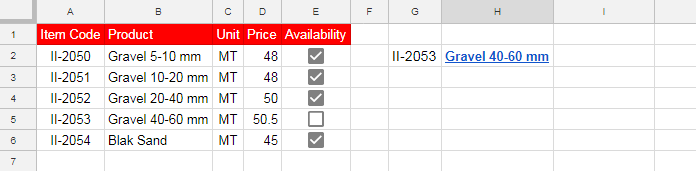
Assume you have a dataset containing item codes, product names, units, unit prices, and availability in columns A to E. You want to VLOOKUP a product by item code and create a clickable link that jumps to the corresponding cell in the product column.

Dataset Structure (Columns A to E):

Item Code	Product	Unit	Price	Availability
II-2050	Gravel 5-10 mm	MT	48	✅
II-2051	Gravel 10-20 mm	MT	48	✅
II-2052	Gravel 20-40 mm	MT	50	✅
II-2053	Gravel 40-60 mm	MT	50.5	❌
II-2054	Black Sand	MT	45	✅

Step 1: VLOOKUP Formula

Use the following VLOOKUP formula in cell H2 to fetch the product name based on the item code entered in G2:

=VLOOKUP(G2, A1:E, 2, FALSE)

Whenever you enter a different item code in G2, the product name in H2 updates dynamically.

However, clicking on H2 won’t take you to the product cell in column B. That’s where hyperlinking to the VLOOKUP result comes in.

Creating a Hyperlink to the VLOOKUP Output Cell

Step 2: Find the Cell Address of the VLOOKUP Result

To get the exact cell address where the VLOOKUP result is found, use the CELL function:

=CELL("address", VLOOKUP(G2, A1:E, 2, FALSE))

This returns a result like “$B$5”, which is the absolute cell reference of the matching product.

Issue: We need to remove the dollar signs ($) and sheet name (if any) for a cleaner reference.

Step 3: Remove the Sheet Name and Dollar Signs ($) from the Cell Address

We’ll use REGEXREPLACE to clean up the cell reference:

=REGEXREPLACE(CELL("address", VLOOKUP(G2, A1:E, 2, FALSE)), ".*!|\$", "")

This removes:

Sheet name (if present)
Dollar signs ($) (so the reference remains flexible)

Now, instead of $B$5, the result is B5.

Step 4: Generate a Dynamic Hyperlink to the VLOOKUP Result

Get the URL for a Cell in Google Sheets
- Right-click cell A1 in your sheet. If your lookup table is in a different sheet from where you’re performing the lookup, navigate to the sheet containing the dataset and right-click cell A1.
- Click “View more cell actions” > “Get link to this cell.” This will copy the URL of the cell.
- Paste the generated Google Sheets URL into an empty cell, as we need to modify it. It will look like this: https://docs.google.com/spreadsheets/d/1WEm8c9zY-PSBwS9qa9mOtFlRVxyrA04uj_9WF8bZ3vM/edit?gid=1450785728#gid=1450785728&range=A1
Remove “A1” and replace it with the dynamic cell address formula from step 3:

"https://docs.google.com/spreadsheets/d/1WEm8c9zY-PSBwS9qa9mOtFlRVxyrA04uj_9WF8bZ3vM/edit?gid=1450785728#gid=1450785728&range="&REGEXREPLACE(CELL("address", VLOOKUP(G2, A1:E, 2, FALSE)), ".*!|\$", "")

Now, this URL dynamically updates to link directly to the correct VLOOKUP output cell.

Step 5: Create a Clickable Hyperlink for the VLOOKUP Output

To display the product name as a clickable hyperlink, use the HYPERLINK function. The syntax is:

=HYPERLINK(URL, [link_label])

Where:

URL is the URL from Step 4
link_label is the VLOOKUP formula from Step 1

Here’s the formula:

=HYPERLINK(
   "https://docs.google.com/spreadsheets/d/1WEm8c9zY-PSBwS9qa9mOtFlRVxyrA04uj_9WF8bZ3vM/edit?gid=1450785728#gid=1450785728&range="&REGEXREPLACE(CELL("address", VLOOKUP(G2, A1:E, 2, FALSE)), ".*!|\$", ""), 
   VLOOKUP(G2, A1:E, 2, FALSE)
)

Final Result: Clicking on the product name in H2 will take you directly to its cell in column B.

Why Use a Hyperlink with VLOOKUP?

Time-Saving: No need to manually scroll to the matched value.
Dynamic Updates: The link changes automatically when you enter a new search key.
Improved Navigation: Useful for large datasets where quick lookups are needed.

FAQs

Q: Can I hyperlink to a VLOOKUP result in another sheet?

A: Yes! The formula is already optimized for this. The issue was that the CELL function returns the sheet name of the lookup table, which we don’t want in the hyperlink. The REGEXREPLACE handles this effectively.

Q: What if my dataset is in a different Google Sheets file?

A: If the dataset is in another file, you’ll need to manually construct the hyperlink using that file’s URL and reference the correct range. Unfortunately, you can’t perform a VLOOKUP between two different sheets and jump to the target sheet directly.

Final Thoughts

Now you know how to create a dynamic hyperlink to a VLOOKUP result in Google Sheets! This method saves time, improves navigation, and automatically updates when the search key changes.

Try it out, and let me know if you have any questions in the comments!

Resources

22 COMMENTS

Baloney Sandwitch March 13, 2023 At 2:28 am

Very good. Also, you can use the MATCH function instead of the VLOOKUP to find the destination cell reference.

ameerah July 15, 2022 At 2:26 pm

Hey, I tried this. However, when I repeat the words, it does not work anymore.

Gareth March 23, 2022 At 9:25 am

This is great, thanks!

A little bit simpler if you use MATCH to get just the numeric part of the cell reference and then combine that with the column letter.

Then you don’t need to SUBSTITUTE anything.

- Prashanth March 25, 2022 At 7:19 am
  
  Hi, Gareth,
  
  That’s correct. But, anyhow, we have to use one Vlookup.
  
  So, I thought to use that formula again for getting the cell address. Then it would be easy for the explanation.
  
Darken October 17, 2020 At 3:23 am

Hi, great work!

I have the following problem with your solution:

I make a copy each year of my sheet (Sheet Blank) and rename it to the current year (Sheet 2019, Sheet 2020, Sheet 2021, etc…) to enter new data for the year. The hyperlinks still jump to the original blank sheet instead of the cell in the current sheet. Is there a way to get the link to the current sheet?

PS: I mean by formula, not having to change the URL manually in every hyperlink each year.

Thanks.

- Prashanth October 17, 2020 At 8:50 am
  
  Hi, Darken,
  
  As you may already know, every sheet has its own unique URLs. I don’t have the formula to extract the URL of a sheet.
  
Dale Harper June 26, 2020 At 3:32 pm

Hi – Your work really is excellent.

Can this above be used in conjunction with other formulas?

I used your tutorial to build what I needed, however, I would now like to add the hyperlink to source location function but am struggling to get it to work:

=CELL("address",ARRAYFORMULA(IFERROR(INDEX('2 - Alpha-Date Order'!I$2:I,SMALL(IF(B3='2 - Alpha-Date Order'!A3:A,ROW('2 - Alpha-Date Order'!A3:A)-1),$D$1)))))

- Prashanth June 27, 2020 At 10:14 am
  
  Hi, Dale Harper,
  
  Please remove the below formula parts from your above formula and the corresponding two closing brackets.
  
  ARRAYFORMULA(IFERROR(
  
  Please let me know whether it works or not. If not, I’ll publish a new tutorial ASAP to help you and other readers to address the issue.
  
  The ArrayFormula supports the non-array IF function. It’s not necessary to use when using the IF inside Index. The ArrayFormula would cause issue in the CELL function.
  
Donna June 22, 2020 At 3:14 pm

How to get the link if the list is on an external sheet?

Nereida May 1, 2020 At 7:07 pm

Hi Prashant,

First of all, many thanks for your contributions! You help me learn a lot 🙂

So, for your reference, I am a Google Sheets user from SPAIN (Windows & Firefox), and have noticed that where your formulas use “,” I have to use “;” to separate arguments. I am not sure if there are other differences I may not be aware of.

That said… I’ve tried this wonderful idea but it does not work 🙁

So maybe you can help?

If I pass this:

=CELL("address";VLOOKUP(B3;AUX!I2:M20;2;FALSE))

Then the output is #N/A [ “Argument must be a range”]

Checking the function help it says “address” output is the absolute reference of the first left cell from the RANGE provided as the second argument…

The output of VLOOKUP, or HLOOUP for that matter, is the content of the cell, of course, then, it is not a range.

Hopefully, you can help with this.

Thanks!

- Prashanth May 2, 2020 At 3:40 pm
  
  Hi, Nereida,
  
  I have tested and your formula returns a proper cell address. The Vlookup + Hyperlink formula for your region, as per your explanation (I’ve read between lines), might be this.
  
  =hyperlink( "use_cell_Aux!A1_link_as_instructed"& substitute( substitute( CELL("address";VLOOKUP(B3;Aux!I2:M20;2;FALSE));"Aux!";""); "$";""); VLOOKUP(B3;Aux!I2:M20;2;FALSE) )
  
  Please replace use_cell_Aux!A1_link_as_instructed in the formula.
  
  If this is not helpful, you can copy my example sheet (link already left within the post) and convert its Locale to yours from that sheet File > Spreadsheet settings > Locale > Spain.
  
  To know more about changes in the formula due to Locale, please read this guide – How to Change a Non-Regional Google Sheets Formula.
  
  - I November 5, 2020 At 10:55 am
    
    I too have this issue. I can replicate your example in the same sheet, different tabs, but when I go to apply this on a separate tab, I also get #N/A [ “Argument must be a range”] when I split out the "=CELL("...) formula for testing. When I apply the whole formula, it produces the right text result in the cell, but it does not apply the hyperlink. Strange…
    
    - Prashanth November 5, 2020 At 1:00 pm
      
      Can I have a look at your sheet?
      
      If it doesn’t contain sensitive or personal data, consider sharing the link with you reply below (it won’t be published).
      
    - Prashanth November 5, 2020 At 1:01 pm
      
      Can I have a look at your sheet?
      
      If it doesn’t contain sensitive or personal data, consider sharing the link with your reply below (it won’t be published).
      
Bohdan April 16, 2020 At 2:14 am

Hello!

I’ve been searching for that !!
I did as you wrote, but it doesn’t recognize it as the right formula.
Some mistakes were found.

My case is:
I have a Master Sheet where I put all my data.
There are a couple of sheets that query data from that Master Sheet.
I need to jump to any cell in the Master Sheet to edit it.

- Prashanth April 16, 2020 At 9:21 am
  
  Hi, Bohdan,
  
  To help you I have included a sample sheet. You can find that at the very end of the post.
  Cheers!
  
Manuel December 17, 2019 At 2:22 pm

Hi,

Thanks for sharing.

Unfortunately, when I reference a cell in another tab of the sheet, it goes to the other tab by clicking BUT not the referenced cell as it says that the link area has been deleted…

- Prashanth December 17, 2019 At 5:44 pm
  
  I think I can correct it. Can you replicate the problem in another file and share that with me?
  
David Moore November 26, 2019 At 4:04 am

This is great – I’m forever searching back through sheets to find the source!
Can this also be made to work in an arrayformula? (as all my vlookups do, better than index-match….)

- Prashanth November 26, 2019 At 9:43 am
  
  Hi, David,
  
  My formula won’t work with a Vlookup array. The reason is the CELL function which I have used to find the cell address of the Vlookup result cell.
  
  Best,
  
Ellen Guldan July 25, 2019 At 11:39 pm

OMG, I have been looking for this for weeks. You solved all my problems today!! I have to say I did not expect to find it paired with “Vlookup” in the title, so possibly I had overlooked it–I use index match myself (and by doing so, avoid the need for the cell function in the formula). THANK YOU
THANK YOU
THANK YOU!

- Prashanth July 26, 2019 At 8:58 am
  
  Hi, Ellen,
  
  Welcome!
  
  Thanks for the feedback!