


")


")

")
")
 in Excel & Google Sheets")


To find the column header of the min value in Google Sheets, you may need different formulas depending on whether you want to include or exclude zero.
For example, if you are identifying the employee with the least sales in a day, you might want to include zero to capture employees with no sales. However, if you are tracking the number of hours students spent on a project, you might want to exclude zero since it may indicate no participation.
Below, I provide two formulas for finding the column header of the min value in Google Sheets. Choose the one that fits your needs.
Find the Column Header of Min Value Including Zero
Assume five employees are working under you, and you want to analyze their daily sales to identify the lowest performer each day.
Here is a sample dataset in the range A1:F10.
| Amy | Dave | Maxine | Malcolm | Edgar | |
| 10/6/21 Thu | 3 | 1 | 5 | 3 | 8 |
| 11/6/21 Fri | 6 | 2 | 5 | 3 | 4 |
| 12/6/21 Sat | |||||
| 13/6/21 Sun | |||||
| 14/6/21 Mon | 2 | 5 | 4 | 1 | 1 |
| 15/6/21 Tue | 10 | 0 | |||
| 16/6/21 Wed | 3 | 3 | 4 | 1 | 2 |
| 17/6/21 Thu | 1 | ||||
| 18/6/21 Fri | 6 | 4 |
The employee names are in the column headers (row 1), and their sales figures are in the corresponding rows below.
Use the following formula in cell H2 and drag it down to apply it to each row. This will return the column header of the min value for each day.
=TEXTJOIN(", ", TRUE, IFNA(FILTER($B$1:$F$1, IF(B2:F2="", NA(), B2:F2)=MIN(B2:F2))))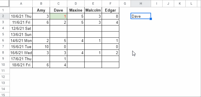
Column Header of Min Value – Non-Array Formula
When using this formula, replace:
$B$1:$F$1with the header row reference.B2:F2with the range where you want to find the min value.
How This Formula Works
FILTER($B$1:$F$1, IF(B2:F2="", NA(), B2:F2)=MIN(B2:F2))- The FILTER function selects the headers from
$B$1:$F$1where the condition evaluates to TRUE. IF(B2:F2="", NA(), B2:F2)=MIN(B2:F2)(condition):- This converts empty cells to
#N/A. - It then checks where values match the minimum value in the row.
- Ensures that empty rows or rows where the min value is zero are not incorrectly filtered.
- This converts empty cells to
- IFNA removes
#N/Aerrors from empty rows (filter result). - TEXTJOIN joins multiple headers if there are ties for the min value.
Converting to an Array Formula
Instead of dragging the formula down, use this array formula in H2 to apply it across all rows:
=BYROW(B2:F10, LAMBDA(row_, TEXTJOIN(", ", TRUE, IFNA(FILTER(B1:F1, IF(row_="", NA(), row_)=MIN(row_))))))This converts the formula into a custom LAMBDA function that applies row-wise using BYROW.
row_represents the current row being processed.- The function dynamically finds the min value for each row and returns the corresponding column header.
Find the Column Header of Min Value Excluding Zero
Using the same sample data, this formula finds the column header of the min value while ignoring zero.
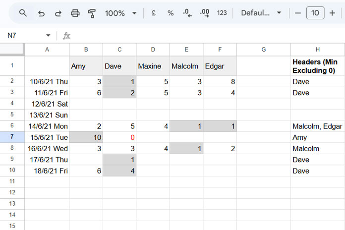
Use this formula in cell H2:
=TEXTJOIN(", ", TRUE, IFNA(FILTER($B$1:$F$1, IF(B2:F2=0, NA(), B2:F2)=MINIFS(B2:F2, B2:F2, ">0"))))Drag it down to apply it to all rows.
How This Formula Differs
Compared to the earlier formula:
IF(B2:F2=0, NA(), B2:F2): Replaces zeros and empty cells with#N/A, ensuring they are ignored.MINIFS(B2:F2, B2:F2, ">0"): Finds the min value greater than zero.- FILTER then returns headers for values matching the min (non-zero) value.
- TEXTJOIN combines multiple headers if there are ties.
Array Formula Version
To avoid dragging the formula down, use this array formula in H2:
=BYROW(B2:F10, LAMBDA(row_, TEXTJOIN(", ", TRUE, IFNA(FILTER(B1:F1, IF(row_=0, NA(), row_)=MINIFS(row_, row_, ">0"))))))This applies the LAMBDA function row-wise, finding the min non-zero value and returning the corresponding column headers.
Resources
- Find the Column Header of the Max Value in Google Sheets
- Find Max N Values in a Row and Return Headers in Google Sheets
- Lookup and Retrieve Column Headers in Google Sheets
- Search Across Columns and Return the Header in Google Sheets
- Get the Headers of the First Non-Blank Cell in Each Row in Google Sheets
- Get the Header of the Last Non-Blank Cell in a Row in Google Sheets