Average by Month in Google Sheets (Formula Options)

In Google Sheets, you might often want to calculate averages by month. This tutorial covers different ways to do that—including how to average by:

Month number (e.g., 1, 2, 12)
Month and year (e.g., 01-2020)
Month name (e.g., Jan)
Month name and year (e.g., Jan 2020)

Sample Data

We have the following sample data in range A1:B:

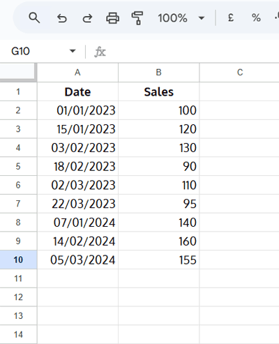
Google Sheets table showing sample sales data across multiple months and years for monthly averaging examples

Let’s look at how to calculate averages by month in Google Sheets.

Comparison Table: Which Method Should You Use?

Method	Pros	Cons	Best For
AVERAGEIF	Simple, intuitive, readable	Requires helper column	Most everyday use cases
QUERY	Tabular output, great for reports	Harder formatting, less flexible	Dashboards and summaries
MAP + LAMBDA	No dragging, very dynamic	More advanced	Automating across conditions
Pivot Table	No formulas required	Less control over formatting	Quick summaries for end users

Average by Month Using Month Numbers (1–12)

Step 1: Extract unique months

=SORT(UNIQUE(MONTH(TOCOL(A2:A, 3))))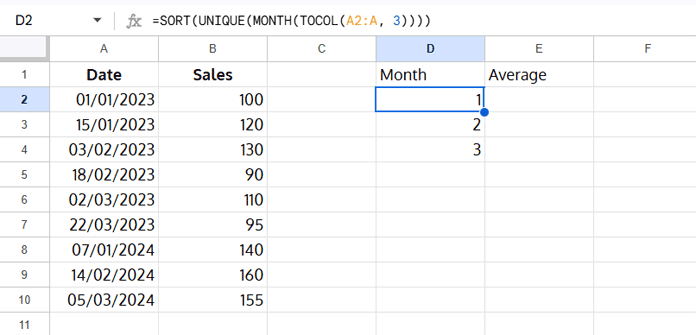

Google Sheets formula in D2 extracting sorted unique month numbers using TOCOL, MONTH, UNIQUE, and SORT

TOCOL removes empty cells
MONTH extracts the month number
UNIQUE removes duplicates
SORT arranges months in ascending order

Step 2: Calculate monthly average

=ArrayFormula(AVERAGEIF(MONTH($A$2:$A), D2, $B$2:$B))

Drag this down alongside the month numbers.

Output:

Animated GIF showing AVERAGEIF formula being dragged down to calculate monthly averages by month number in Google Sheets

Note: The following examples don’t include screenshots, but they follow the same two-step structure as the previous section. In each case, the Step 1 formula (to extract unique labels) goes in cell D2, and the Step 2 formula (to calculate the average) goes in cell E2—unless mentioned otherwise.

Average by Month and Year

Use this method if your data spans more than one year.

Step 1: Extract month and year

=ArrayFormula(UNIQUE(TEXT(SORT(TOCOL(A2:A, 3)), "MM-YYYY")))

TEXT(..., "MM-YYYY") formats the date

Step 2: Calculate average

=ArrayFormula(AVERAGEIF(TEXT($A$2:$A, "MM-YYYY"), D2, $B$2:$B))

Drag this down to apply the formula for each month-year value.

Output:

Month & Year	Average
01-2023	110
02-2023	110
03-2023	102.5
01-2024	140
02-2024	160
03-2024	155

Average by Month Name in Google Sheets

Step 1: Extract month names

=ArrayFormula(UNIQUE(TEXT(SORT(TOCOL(A2:A, 3)), "MMM")))

You can use "MMMM" for full month names.

Step 2: Calculate average

=ArrayFormula(AVERAGEIF(TEXT($A$2:$A, "MMM"), D2, $B$2:$B))

Match the format (MMM or MMMM) in both formulas.

Drag this down to get the average for each month.

Output:

Month	Average
Jan	120
Feb	126.6666667
Mar	120

Average by Month and Year in “Jan 2020” Format

Step 1: Extract month name and year

=ArrayFormula(UNIQUE(TEXT(SORT(TOCOL(A2:A, 3)), "MMM YYYY")))

Step 2: Calculate average

=ArrayFormula(AVERAGEIF(TEXT($A$2:$A, "MMM YYYY"), D2, $B$2:$B))

Copy or drag the formula down to fill averages for each label.

Output:

Month & Year	Average
Jan 2023	110
Feb 2023	110
Mar 2023	102.5
Jan 2024	140
Feb 2024	160
Mar 2024	155

Average by Month Using a Pivot Table

If you prefer not to use formulas, you can easily calculate monthly averages using a pivot table:

Select your dataset (A1:B10).
Go to Insert > Pivot table.
In the popup, choose where to place the pivot table—either in a new sheet or in an existing sheet (specify the cell location).
In the Pivot Table Editor:
- Add Date to Rows.
- Add Sales to Values and change the summarize function to AVERAGE.
Right-click on any date in the pivot table.
Select Create Pivot Date Group > Month or Year-Month, depending on your preference.

GIF showing date grouping by Year-Month and resulting average values in a Google Sheets pivot table

This method gives you a clean monthly summary without writing any formulas.

Additional Tips

Google Sheets’ QUERY function also supports monthly and yearly aggregation.

Average by Month using QUERY

=QUERY(A2:B, "SELECT MONTH(Col1)+1, AVG(Col2) WHERE Col1 IS NOT NULL GROUP BY MONTH(Col1)+1 LABEL MONTH(Col1)+1 'Month', AVG(Col2) 'Average'")

Output:

Month	Average
1	120
2	126.6666667
3	120

Average by Month and Year using QUERY

=QUERY(A2:B, "SELECT MONTH(Col1)+1, YEAR(Col1), AVG(Col2) WHERE Col1 IS NOT NULL GROUP BY MONTH(Col1)+1, YEAR(Col1) ORDER BY YEAR(Col1), MONTH(Col1)+1 LABEL MONTH(Col1)+1 'Month', YEAR(Col1) 'Year', AVG(Col2) 'Average'")

Output:

Month	Year	Average
1	2023	110
2	2023	110
3	2023	102.5
1	2024	140
2	2024	160
3	2024	155

Final Thoughts

We’ve explored multiple ways to calculate the average by month in Google Sheets, including:

AVERAGEIF with month, month-year, and month name formats
QUERY-based summaries
Pivot tables for quick no-formula solutions

Automate Monthly Averages Using MAP and LAMBDA

If you don’t want to drag the formula down manually for each month or month-year, you can use the MAP function to automate it.

Here’s how to convert a drag-down formula into a dynamic one:

=MAP(criteria_range, LAMBDA(r, your_formula_here))

Replace criteria_range with your list of month numbers, names, or formatted labels (e.g., D2:D).
In your your_formula_here, which you’d normally drag down using a reference like D2, replace that reference with r—this allows the MAP function to apply the logic across all values in your criteria_range.

Example formula in cell E2:

=MAP(D2:D4, LAMBDA(r, ArrayFormula(AVERAGEIF(MONTH($A$2:$A), r, $B$2:$B))))

This tells Google Sheets to automatically apply the formula to each item in your criteria range—no manual dragging required.