We can convert almost every non-array formula to an array formula in Google Sheets. The Lambda functions made it possible. We can use an array formula now to sum the sets or groups of every n values in Google Sheets.

Assume you have daily data entered in a column or row. You want the sum of weekly data, not based on dates but based on cell ranges.

For example, get the sum of A1:A7 in B1, A8:A14 in B2, A15:A21 in B3, and so on.

We have already seen how to use a drag-down (non-array) formula for this in my following tutorial: How to Sum Every N Cells to the Right or Bottom in Google Sheets.

When I wrote that tutorial, the scenario was different from now. We didn’t have the Lambda functions at that time.

Not only Lambda; we were missing powerful lookup functions like XLOOKOUP and XMATCH; and functions for selecting and wrapping values like CHOOSEROWS, CHOOSECOLS, etc.

That doesn’t mean we had left with no option to write an array formula to sum sets of every n values at that time. We had an MMULT approach which I used for the average calculation: Array Formula to Return Average of Every N Cells in Google Sheets.

Since we now have a much simpler way of converting non-array formulas to array formulas (LAMBDA), we will use it instead of MMULT.

Array Formula to Sum Sets of Every N Values in a Column

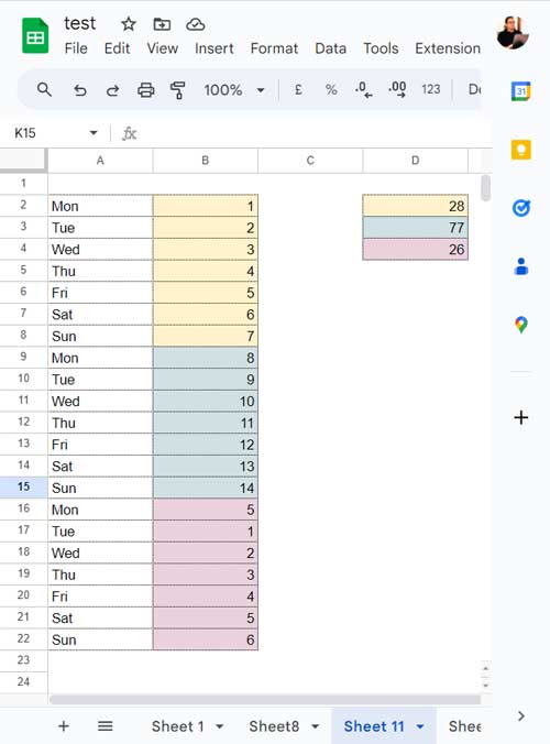
For example, assume we have our daily data in columns A and B, where A contains weekdays and weekends in multiple sets and amounts in column B.

Then we can use the following array formula in another blank column, for example, in cell D2 to get the sum of every set of 7 values in B2:B.

=let(range,B2:B,n,7,n_sets,rounddown(counta(range)/n),map(sequence(n_sets,1,1,n),lambda(r,sum(chooserows(range,sequence(n,1,r))))))

How do I use this array formula to sum every set of 7 values in my Google Sheets?

You may have data in different ranges. Also, the n may not be 7. So, understanding the parameters in the formula may help you.

You require to modify two parameters: B2:B and 7. B2:B is the numerical range, and 7 is the n which defines the number of values in each set.

Notes

1. Use open range (B2:B for B2:B100) to get the sum of every set of n values.
2. If the number of values in the last bin (set) is less than n, the formula will omit that. So stick to point # 1.

How Does the Array Formula Sum Every Set of N (7) Values?

Here is the logic and formula explanation.

Basic Form

Here is the basic form of the formula after removing the LET and its assigned names. LET allows storing intermediate calculations, values, or defining names inside a formula in Google Sheets.

=map(sequence(rounddown(counta(B2:B)/7),1,1,7),lambda(r,sum(chooserows(B2:B,sequence(7,1,r)))))

Try this formula in cell D2. It will work equally well. Then why should I use LET in the original formula above?

It’s because LET makes the formula easy to read and edit. In some cases, it can enhance the performance by avoiding repetitive calculations.

Formula Logic and Explanation

Here is the core part of the array formula that sums sets of every 7 values in Google Sheets.

sum(chooserows(B2:B,sequence(7,1,r)))

Other than SUM, there are two functions in use: CHOOSEROWS and SEQUENCE, and knowing the syntax of the latter function is useful.

Syntax of SEQUENCE: SEQUENCE(rows, [columns], [start], [step])

In the formula part;

rows: 7

columns: 1

start: r

We haven’t specified the step value. So the formula differs the sequence numbers by 1.

The start value is the key which is named ‘r’. If r=1, the SEQUENCE returns the numbers 1 to 7. So the CHOOSEROWS returns the first set of 7 values. If r = 8, the SEQUENCE returns the numbers 8 to 14. So the CHOOSEROWS returns the second set of 7 values. This pattern continues.

The MAP Lambda feeds 1, 8, 15, … to r. For that, it uses another part of the formula, and here it is.

sequence(rounddown(counta(B2:B)/7),1,1,7)

rows: rounddown(counta(B2:B)/7)

columns: 1

start: 1

step: 7

It returns the numbers 1, 8, 15, etc., because of the step value 7.

The Formula for Row Range

In the above formula, we have used MAP Lambda instead of BYROW. So the formula works equally well in a row range also.

But we require one change in the formula. We must replace CHOOSEROWS with CHOOSECOLS. Also, don’t forget to use open range, and here is one example.

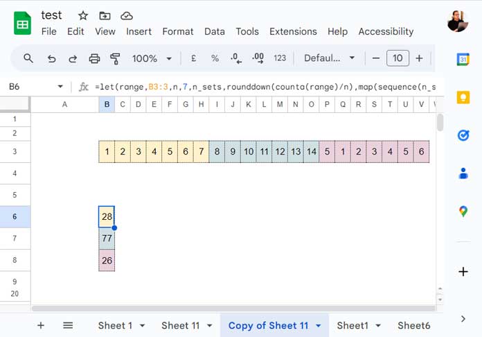
Array Formula to Sum Sets of Every 7 Values in a Row in Google Sheets:

=let(range,B3:3,n,7,n_sets,rounddown(counta(range)/n),map(sequence(n_sets,1,1,n),lambda(r,sum(choosecols(range,sequence(n,1,r))))))

Wrap the formula with TRANSPOSE if you want the result also in rows.

That’s all. Thanks for the stay. Enjoy!