


The AMORLINC function in Google Sheets calculates depreciation for a period using linear depreciation, as defined in the French accounting system.
In this Google Sheets tutorial, I have included all the necessary tips to help you learn this financial function, such as:
- AMORLINC syntax
- Formula examples
- Manual calculation
- An AMORLINC depreciation chart
The linear depreciation method is the most widely used method to calculate depreciation for tangible assets.
For example, if an asset has an initial cost of $6,000.00 and a residual (scrap) value of $1,500.00 after 3 years (its useful life), then each year, $1,500.00 [=(6000-1500)/1/3] will be written off as depreciation. In this case, 1/3 is the depreciation rate.
In Google Sheets, you can use the SLN (Straight Line Depreciation) function for these types of calculations.
=SLN(6000,1500,3)However, the AMORLINC function is slightly different. It returns the prorated depreciation if the asset was purchased in the middle of a period. I have detailed this under the subtitle “How to Create a Depreciation Table Without AMORLINC in Google Sheets” below.
Syntax and Arguments
Syntax of the AMORLINC Function in Google Sheets:
AMORLINC(cost, purchase_date, first_period_end, salvage, period, rate, [basis])Arguments:
cost: The acquisition/purchase cost of the asset.purchase_date: The date on which the asset was acquired/purchased.first_period_end: The end date of the first depreciation period.salvage: The scrap value of the asset at the end of its useful life.period: The period for which to calculate depreciation. The initial period is 0.rate: The annual depreciation rate, expressed as a percentage or as a decimal.- The
rateargument in the AMORLINC function is the annual depreciation rate, expressed as a percentage or as a decimal. For example, if you want to use a 25% depreciation rate, you can enter25%or0.25in the formula.
- The
basis: An optional argument that specifies the day count convention to use. It can be one of the following values:
| Basis | Day Count Methods | Remarks |
| 0 | 30/360. 30-day months and 360-day years (NASD) | Default |
| 1 | Actual/Actual. | For calculation based on the actual number of days between the specified dates and the actual number of days in the intervening years. |
| 2 | Actual/360. | |
| 3 | Actual/365. | |
| 4 | 30/360. European. |
How to Use the AMORLINC Function in Google Sheets
Example of the AMORLINC function in Google Sheets:
Asset: Purchased on June 1, 2018 for $6,000.00 and depreciated at 25% per year.
Depreciation expense for the first period ending on December 31, 2018: $1,500.00
Input values and AMORLINC formula:
| Input | Values |
| Cost | $6,000.00 |
| Purchase date | June 1, 2018 |
| First-period end date | December 31, 2018 |
| Salvage value | $1,500.00 |
| Period | 1 |
| Depreciation rate | 25% |
| Day count basis | 1 (Actual/Actual) |
Formula:
=AMORLINC(6000, DATE(2018,6,1), DATE(2018,12,31), 1500, 1, 0.25, 1)When using the AMORLINC function with hard-coded input values (instead of cell references), use the DATE function to specify the purchase date and first-period end date to avoid unintentional errors. The syntax of the DATE function is: DATE(year, month, day).
How to Create a Depreciation Table and Chart in Google Sheets Using the AMORLINC Function
Enter the above input values, except for the period, in the cell range B2:B8 to create a depreciation table. We will use periods from 0 to 4 in D2:D6.
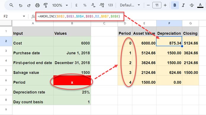
As mentioned above, the initial period of depreciation is 0. The depreciation table above shows the depreciation of the asset from period 0 with the day count basis set to Actual/Actual.
To create the depreciation table in Google Sheets, I used the following AMORLINC formula in cell F2 and copied it down to cell F6:
=AMORLINC($B$2,$B$3,$B$4,$B$5,D2,$B$7,$B$8)In this formula, I kept the cell reference D2 relative because I wanted to change the “period” accordingly when dragging the formula down (D2 to D3 and so on).
I have two more formulas in the Sheet.
Cell G2 contains the formula =E2-F2 (asset value – depreciation), which was copied down.
Cell E2 contains the purchase cost of the asset. In cell E3, I used the formula =G2 and dragged it down to get the asset value in each period.
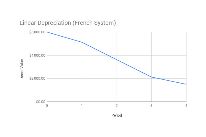
How do I create a Linear Depreciation (French System) Chart from the above table in Google Sheets?
- Select the range D1:E6.
- Click the Insert menu > Chart.
- Under Setup in the Chart editor dialog box in the sidebar, select Line Chart.
How to Create a Depreciation Table Without AMORLINC in Google Sheets
In the above example of using the AMORLINC function in Google Sheets, you can see that I have calculated the depreciation for periods 0, 1, 2, and 3. Here is how to calculate them using the YERFRAC function (which extracts the number of years between two dates) and operators.
Depreciation in the Initial Period
The initial period is 0, and the depreciation calculation for this period is:
cost * rate * YEARFRAC(purchase_date,first_period_end, day_count_convention)Depreciation for Period 0:
=6000*0.25*YEARFRAC(DATE(2018,6,1),DATE(2018,12,31),1) // returns $875.34Depreciation in the Subsequent Periods (Whole Periods Only)
For the first and second periods, which are whole periods according to the example, the calculation is cost * rate, which will return $1,500.00.
=6000*0.25 // returns $1500.00Depreciation in the Final Period (Fractional Period)
In the third period, which is the final period in my example, the formula will be cost - salvage - cumulative depreciation amount.
=6000-1500-875.34-1500-1500 // returns $624.66