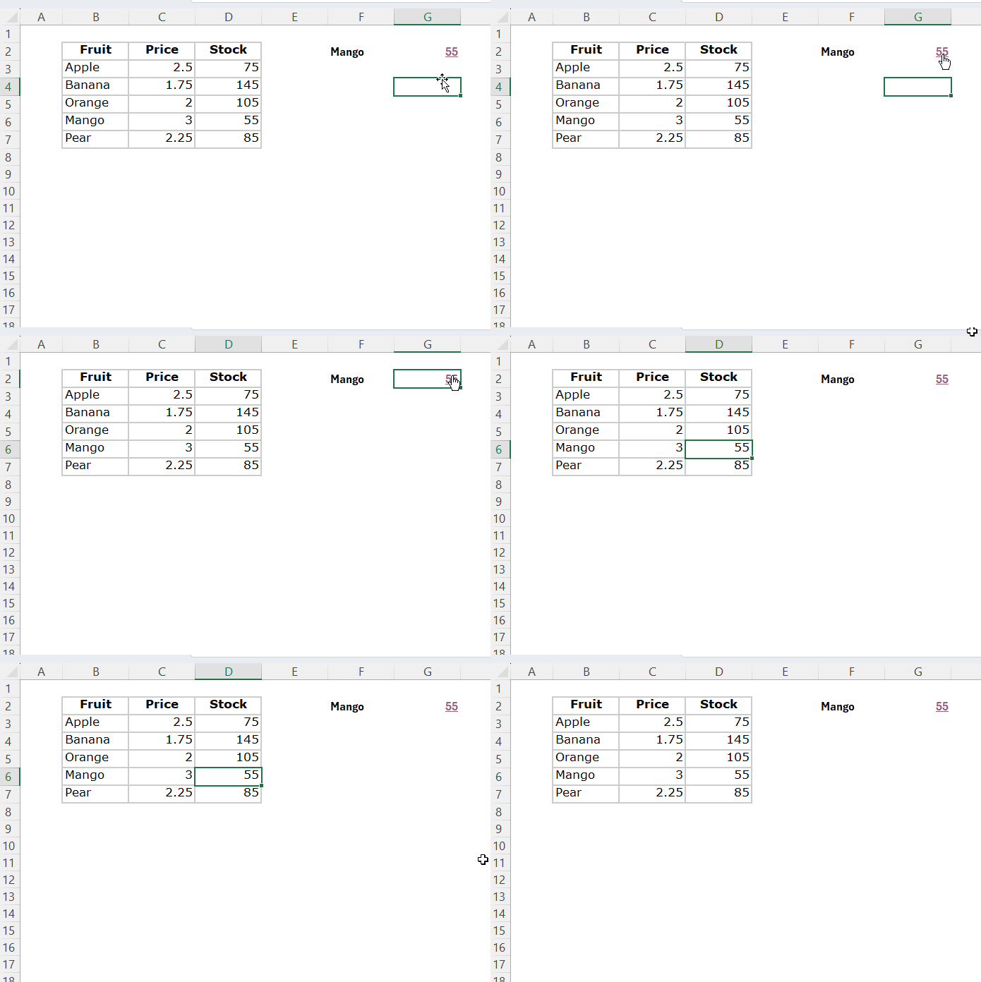
In Excel, we can create a hyperlink to jump to the VLOOKUP result cell by using the CELL, INDEX, MATCH, and HYPERLINK functions. This is similar to how you can jump to the current date cell in Excel.
Where is this useful?
Imagine you want to look up the price of a fruit and modify it. In such a case, this approach can quickly take you to the VLOOKUP result cell, allowing you to make edits easily.
Here is the formula to jump to the VLOOKUP result cell in Excel:
=HYPERLINK("#"&CELL("ADDRESS", INDEX(table_array, MATCH(lookup_value, INDEX(table_array, 0, 1), 0), col_index_num)), VLOOKUP(lookup_value, table_array, col_index_num, 0))You can easily modify this formula for your range, as you only need to adjust the arguments, similar to how VLOOKUP works:
lookup_value– The value you want to search for.table_array– The range where the lookup will occur.col_index_num– The column number from which to return the result.
Example of Jumping to the VLOOKUP Result Cell in Excel
Assume you have the following table in the range B2:D7, which contains fruit names, prices, and stock quantities in columns B, C, and D, respectively.
Now, let’s say you want to create a hyperlink that will take you to the cell where the quantity (stock) of “Mango” is located.
Enter “Mango” in cell F2, and use the following formula in cell G2:
=HYPERLINK("#"&CELL("ADDRESS", INDEX(B2:D7, MATCH(F2, INDEX(B2:D7, 0, 1), 0), 3)), VLOOKUP(F2, B2:D7, 3, 0))Where:
lookup_value– F2table_array– B2:D7col_index_num– 3
This formula allows you to jump to the VLOOKUP result cell in Excel, specifically to the stock quantity of the fruit specified in F2.

Formula Breakdown
This is essentially a HYPERLINK formula in Excel, which consists of two parts:
HYPERLINK(link_location, friendly_name)The friendly_name is the link label, which is your VLOOKUP formula itself:
VLOOKUP(F2, B2:D7, 3, 0)So, how do we jump to this VLOOKUP result cell? In other words, how do we specify the link_location?
The link_location is a combination of the CELL, INDEX, and MATCH functions, as shown here:
"#"&CELL("ADDRESS", INDEX(B2:D7, MATCH(F2, INDEX(B2:D7, 0, 1), 0), 3))Breakdown of Components:
INDEX(B2:D7, 0, 1): This extracts the first column in thetable_array(i.e., B2:B7).MATCH(F2, …, 0): This matches thelookup_valuein cell F2 against the column obtained from the previous INDEX.INDEX(B2:D7, …, 3): This offsets the number of rows returned by MATCH within thetable_arrayB2:D7 and offsets 3 columns (the column index number).
This approach is a workaround to return the result of the VLOOKUP since we can’t directly extract the cell reference from the VLOOKUP result.
CELL("ADDRESS", …): The CELL function returns the cell address in text format."#"&…: This combines the “#” symbol with the address returned by the CELL function to create thelink_location.
This way, we can create a hyperlink to jump to the VLOOKUP result cell in Excel. When you replace the lookup_value in cell F2, the VLOOKUP result will refresh, along with the hyperlink.
Resources
- How to Create a Clickable Next Button in Excel
- How to Jump to Specific Sheet Tab in Google Sheets
- Hyperlink to Jump to Current Date Cell in Google Sheets
- Jump to the Last Cell with Data in a Column in Google Sheets
- Search Value and Hyperlink Cell Found in Google Sheets
- Create a Hyperlink to the VLOOKUP Output Cell in Google Sheets
- How to Create a Hyperlink to an Email Address in Google Sheets
- Hyperlink Max and Min Values in Column or Row in Google Sheets
- Hyperlink to Index-Match Output in Google Sheets
- Hyperlink Calendar Dates to Events in Google Sheets


