The key to mastering the Excel BYROW function lies in understanding the utilization of the standalone LAMBDA function.
Why is BYROW called a LAMBDA helper function in Excel?
BYROW enables the application of an unnamed LAMBDA function, coded for a single row, to an array separated by row. Consequently, it’s referred to as a helper function, despite both being independent functions.
One thing is clear: we must initially create a standalone LAMBDA function (a reusable function without a name) for a row—for example, SUM, AVERAGE, MIN, MAX, PRODUCT. Then, we use the BYROW function to apply this LAMBDA function to each row within the range.
If you grasp this technique, mastering the BYROW Lambda helper function in Excel becomes easy.
Note: BYROW and LAMBDA functions may not be available in all versions of Excel.
Sample Data
We have sample data in cell range A1:M5, representing car sales in four regions over a year. The month names are in row 1, and the regions are in column 1.
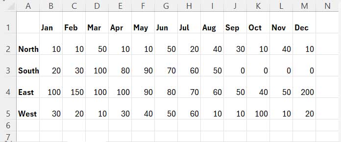
So the range for aggregations is B2:M5, excluding the labels in the first row and column. We will write an unnamed LAMBDA function for the row range B2:M2 and then utilize BYROW to apply it to each row within the range B2:M5.
This is the best approach to understanding the BYROW Lambda helper function in Excel.
Step #1: Coding the Unnamed LAMBDA Function
The following formula will return the total sales of cars in the North region, which is in the range B2:M2:
=SUM(B2:M2)When coding the BYROW formula step by step, remove the “=” sign in front of the formula to make it just a string. We will add it once we complete the steps.
So the string is “SUM(B2:M2)”.
Let’s use a meaningful name to replace B2:M2 in the formula (string). Since it’s sales data for a region, I’ll use the name “sales_per_region”. If you use multiple words, either use an underscore to separate them, or enter them without spaces such as “SalesPerRegion”. This may help avoid unsupported names in use.
SUM(sales_per_region)This will serve as the calculation within a LAMBDA function.
The syntax (adapted for the BYROW Function) of the Excel LAMBDA function is as follows:
LAMBDA(parameter1, calculation)We already have the calculation part, which is “SUM(sales_per_region)”. Use the name “sales_per_region” in the calculation as parameter1. Here is the unnamed LAMBDA function.
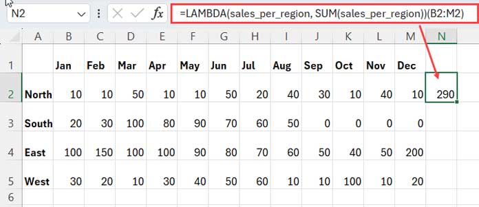
LAMBDA(sales_per_region, SUM(sales_per_region))Right now, it’s just a string and won’t work. If you want to test it, you need to pass the reference B2:M2 to “sales_per_region” as follows:
=LAMBDA(sales_per_region, SUM(sales_per_region))(B2:M2)This is equivalent to =SUM(B2:M2).
But when coding the BYROW formula in Excel, we don’t need to pass the reference like this. We will use BYROW for that. So for the time being, keep it as a string.
Step #2: Coding the BYROW Formula
The Excel BYROW function recognizes the LAMBDA as values. Here is the syntax of the BYROW function in Excel:
=BYROW(array, lambda)Where:
array: An array or range to be separated by a row.lambda: A LAMBDA that takes a row as a single parameter and calculates one result.
In our example, the array to be separated by row is B2:M5, and the lambda is LAMBDA(sales_per_region, SUM(sales_per_region)).
Here is our first BYROW formula to sum by row in Excel:
=BYROW(B2:M5, LAMBDA(sales_per_region, SUM(sales_per_region)))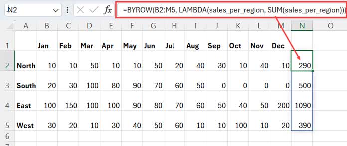
Feel free to replace SUM with MIN, MAX, AVERAGE, PRODUCT, SMALL, LARGE, etc. These functions produce a single result, and you will get MIN, MAX, AVERAGE, PRODUCT, SMALL, LARGE… by row.
Note: When replacing SUM with SMALL or LARGE, please follow their syntax. For example, you can replace SUM(sales_per_region) with SMALL(sales_per_region), 1).
Formula Examples to Excel BYROW Function
Once you’ve learned the Excel BYROW function, you can leverage it for advanced calculations.
For example, in the sample data provided above, if you need to find the month names in which the maximum sales occurred, you can utilize BYROW with functions like XLOOKUP or FILTER.
BYROW with XLOOKUP in Excel
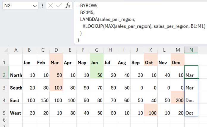
The following formula finds the maximum sales in each row and returns the corresponding header of the first occurrence:
=BYROW(
   B2:M5,
   LAMBDA(
      sales_per_region,
      XLOOKUP(MAX(sales_per_region), sales_per_region, B1:M1)
   )
)
For instance, if the maximum sales in the first row are 50, occurring in March and June, the formula will return the month name “March”. Similarly, for each row, the formula will return the header corresponding to the maximum sales.
The unnamed LAMBDA function for a single row is:
=LAMBDA(sales_per_region, XLOOKUP(MAX(sales_per_region), sales_per_region, B1:M1)) (B2:M2)XLOOKUP searches for the maximum value in sales_per_region and returns the corresponding value in B1:M1 (the header row).
We used BYROW to operate within a range separated by row.
BYROW with FILTER in Excel
In the above example, if you want all the values in the header corresponding to the maximum sales, you may need to use the FILTER function along with the BYROW function in Excel:
=BYROW(
   B2:M5,
   LAMBDA(
      sales_per_region,
      TEXTJOIN(", ", TRUE, FILTER(B1:M1, sales_per_region=MAX(sales_per_region)))
   )
)
In this formula, the LAMBDA function for a single row is as follows:
=LAMBDA(sales_per_region, TEXTJOIN(", ", TRUE, FILTER(B1:M1, sales_per_region=MAX(sales_per_region)))) (B2:M2)The FILTER function filters B1:M1 if sales_per_region equals MAX(sales_per_region). The TEXTJOIN function combines multiple month names if they are returned.
The BYROW function uses the array B2:M5 to execute the unnamed LAMBDA function in each row.
Conclusion
The BYROW function in Excel might seem complex at first glance. However, if you understand the LAMBDA function, you can easily grasp its usage. The above examples align with this principle.
The last two examples illustrate how mastering LAMBDA helper functions opens up powerful possibilities for advanced data manipulation and analysis in Excel.
With practice and patience, you can leverage BYROW to streamline your workflows and perform advanced calculations with ease.
Resources:


