


With the help of two simple custom formulas, we can drop rows and columns by their index number in Google Sheets. One formula is designated for rows, and the other for columns. Additionally, they can be nested. These formulas offer the following features:
- Dropping rows/columns based on index number (where the index numbers denote the row/column position in the data range).
- Dropping rows/columns from the beginning of the range.
- Dropping rows/columns from the end of the range.
As a side note, it’s important to mention that the DROP function is not available in Google Sheets at the time of writing this post.
Drop Rows by Index
Here is the generic formula for drop rows by index in Google Sheets:
=LET(
   range, specify_range_reference,
   seq_r, SEQUENCE(ROWS(range)),
   FILTER(range, NOT(IFNA(XMATCH(seq_r, {row_index}))))
)
In this formula, you need to replace ‘specify_range_reference’ with your data range and ‘row_index’ with the row numbers (index numbers) that you want to drop. Index numbers are:
- Comma-separated, like
5, 8, to eliminate rows 5 and 8. 1, 2, 3to eliminate 3 rows from the beginning of the range.LARGE(seq_r, 1), LARGE(seq_r, 2), LARGE(seq_r, 3)to remove 3 rows from the end.
Here are examples to help you understand how to use my custom formula to drop rows by index in Google Sheets.
Examples
There are 6 rows and 5 columns in our sample data, which is in the range A1:E6. To remove the fourth row in this range, we can use the following formula:
=LET(
   range, A1:E6,
   seq_r, SEQUENCE(ROWS(range)),
   FILTER(range, NOT(IFNA(XMATCH(seq_r, {4}))))
)
Where A1:E6 is the data range (table range) and 4 is the row to drop in the table.
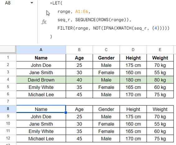
To drop rows 4 and 6, specify it as {4, 6} instead of {4}. If you want to drop the header of the table, replace {4} with {1}. That means you can specify row numbers to eliminate rows from the beginning of the table as well.
How to eliminate rows from the end of a table range in Google Sheets?
The following formula drops the last row in the table:
=LET(
   range, A1:E6,
   seq_r, SEQUENCE(ROWS(range)),
   FILTER(range, NOT(IFNA(XMATCH(seq_r, {LARGE(seq_r, 1)}))))
)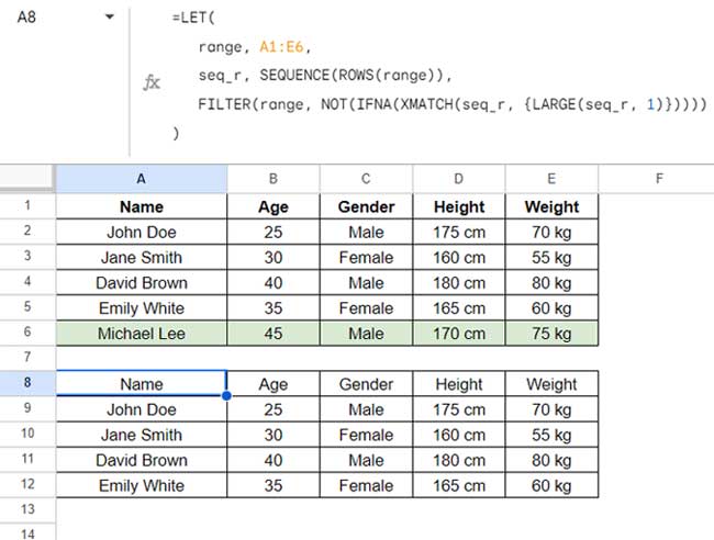
To drop the last two rows, replace {LARGE(seq_r, 1)} with {LARGE(seq_r, 1), LARGE(seq_r, 2)}.
Drop Columns by Index
Here is the generic formula to drop columns by index in Google Sheets:
=LET(
   range, specify_range_reference,
   seq_c, SEQUENCE(1, COLUMNS(range)),
   FILTER(range, NOT(IFNA(XMATCH(seq_c, {column_index}))))
)
In this formula, ‘specify_range_reference’ is your data range, and ‘column_index’ represents the index numbers of the columns that you want to remove. Column index numbers can be:
- Comma-separated, like
2, 4, to drop columns 2 and 4. 1, 2, 3to drop 3 columns from the beginning of the range.LARGE(seq_c, 1), LARGE(seq_c, 2), LARGE(seq_c, 3)to drop 3 columns from the end.
Examples
The usage is similar to dropping rows from the range. Here, you need to consider the column index, where the first column has index number 1.
For example, to remove columns two and three, we can use the following formula:
=LET(
   range, A1:E6,
   seq_c, SEQUENCE(1, COLUMNS(range)),
   FILTER(range, NOT(IFNA(XMATCH(seq_c, {2, 3}))))
)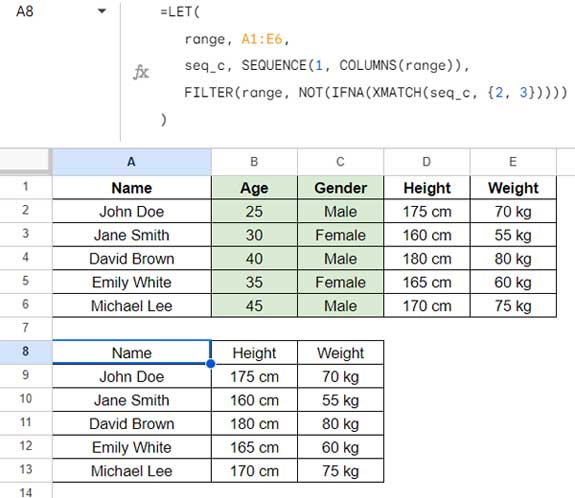
To drop columns from the beginning of the range, for example, the first two columns, replace {2, 3} with {1, 2}.
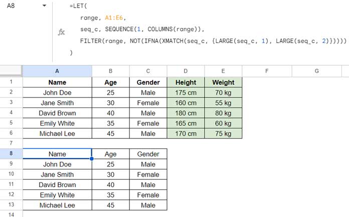
To drop columns from the end, you should specify the column index differently. Use the column index {LARGE(seq_c, 1), LARGE(seq_c, 2)} to remove the last two columns.
=LET(
   range, A1:E6,
   seq_c, SEQUENCE(1, COLUMNS(range)),
   FILTER(range, NOT(IFNA(XMATCH(seq_c, {LARGE(seq_c, 1), LARGE(seq_c, 2)}))))
)
Additional Tip
You can drop rows and columns simultaneously. First, use a formula to remove rows, and then use another formula to remove columns. This will give you two outputs.
Next, cut the second formula and paste it over the physical range, such as A1:E6, in the first formula.
Formula Logic and Explanation
Both the row and column-dropping formulas employ the same logic. They utilize the FILTER function to sift through specified rows or columns within the range.
In both formulas, the SEQUENCE section generates sequential numbers corresponding to rows or columns in the range.
XMATCH then matches these row or column numbers against the user-specified index numbers, returning numbers for matches and #N/A for mismatches. IFNA is used to eliminate these errors.
The NOT function converts numbers to FALSE and blanks returned by IFNA to TRUE. The FILTER function subsequently filters rows matching TRUE.
For a detailed breakdown, let’s consider the following formula, which drops columns two and three in the range A1:E6:
=LET(
   range, A1:E6,
   seq_c, SEQUENCE(1, COLUMNS(range)),
   FILTER(range, NOT(IFNA(XMATCH(seq_c, {2, 3}))))
)
The section SEQUENCE(1, COLUMNS(range)) returns sequence numbers {1, 2, 3, 4, 5}, where 1 in SEQUENCE represents the number of rows in the sequence, and COLUMNS(range) represents the number of columns in the sequence. It is named seq_c.
XMATCH(seq_c, {2, 3}) – The XMATCH function searches these values (sequence numbers) within the columns to be dropped (specified as the array {2, 3}), resulting in the array {#N/A, 1, 2, #N/A, #N/A}.
This outcome occurs because the search keys are {1, 2, 3, 4, 5}, and the lookup range is {2, 3}. The relative positions of the search keys 2 and 3 in the lookup range are 1 and 2, respectively, and other values are not present in the lookup range. We aim to identify the columns containing #N/A, which are columns 1, 4, and 5. IFNA removes these errors, and NOT returns TRUE for those columns and FALSE for others.
The FILTER function filters columns in the range A1:E6 where columns corresponding to TRUE in the XMATCH result array.
That’s all about how to drop rows and columns by index in Google Sheets.