


I have an array formula to get the reverse running total in Google Sheets.
When you have your data sorted from newest to oldest, you may find this very useful over the running total (cumulative sum).
For example, let’s consider the wheat production in Australia from 2010 to 2019 (data from wiki).
In Google Sheets, we can arrange the data in two columns as below.
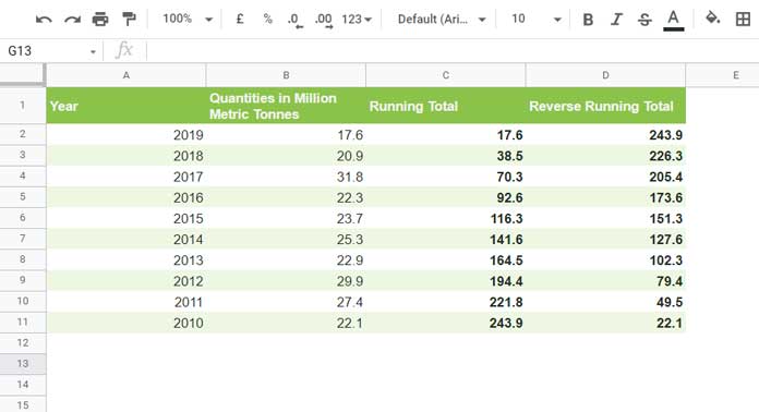
Columns A and B contain years and the quantities of wheat production (million metric tonnes), respectively.
What is important here is the data arranged in descending order (newest to oldest) by the year in column A.
See the values in the cumulative sum columns C and D.
How do they differ?
In column C, you can see the running total calculated from top to bottom, whereas, in column D, the same calculation is from bottom to top.
From column D, you can understand the cumulative wheat production up to that year from each row.
How to calculate the reverse running total in Google Sheets as above in column D?
If you prefer a non-array formula, you can use the below formula in cell D2 and drag it down until row#11.
=sum($B$2:$B)-sum(arrayformula(n($B$1:B1)))But I do have an array formula.
Array Formula for Reverse Running Total in Google Sheets
We will use a SUMIF array formula here.
Syntax:
ArrayFormula(SUMIF(range, criterion, [sum_range]))We have the sum_range to calculate the reverse cumulative sum, which is B2:B. What about range and criterion?
You can find that within the formula below.
Empty the entire column D because we want to insert an array formula in cell D1, which requires an empty column to work without the #REF error.
The below formula is for cell D1.
={"Reverse Running Total";ArrayFormula(If(B2:B="",,SUMIF(sort(row(A2:A),1,0),"<="&sort(row(A2:A),1,0),B2:B)))}The above array formula will return the reverse running total in Google Sheets for the range B2:B.
It has a sheer benefit over its counterpart (non-array).
It uses an open range B2:B. So it will return the reverse running total in all the rows in column D. But, there should be values in column B. Blank rows will be ignored.
Learn the range and criterion used in the formula from the explanation part below.
Update: This will also work ={"Reverse Running Total";ArrayFormula(If(B2:B="",,SUMIF(row(A2:A),">="&row(A2:A),B2:B)))}. But the explanation will be based on the formula above.
Formula Explanation
Let’s remove the unwanted string from the formula, i.e., the header “Reverse Running Total,” and make the ranges closed. Then use a helper column.
So we can shorten the SUMIF formula and make it easily readable.
=ArrayFormula(If(B2:B11="",,SUMIF(C2:C11,"<="&C2:C11,B2:B11)))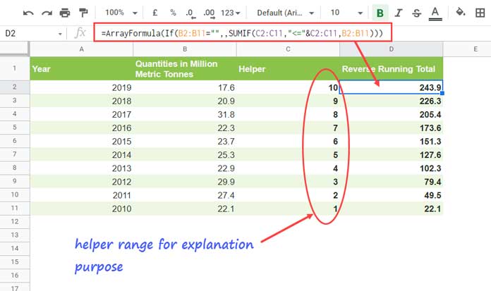
We can split the formula into three parts.
Part 1
ArrayFormula – To help the SUMIF to return an array result. The IF also requires this.
ArrayFormula(Part 2
IF – To limit the output in such rows that contain values in column B.
If(B2:B11="",,Part 3
SUMIF – To return the reverse running total in Google Sheets.
SUMIF(C2:C11,"<="&C2:C11,B2:B11)Note:- The cell range C2:C11 is a temporary helper range for the formula explanation. Please refer to the image above. In the main formula, we have used sort(row(A2:A),1,0) instead.
This formula requires a detailed explanation to understand how the SUMIF returns reverse running total in Google Sheets.
Let’s test the formula in a particular row, for example, in row # 5.
=SUMIF(C2:C11,"<="&C5,B2:B11)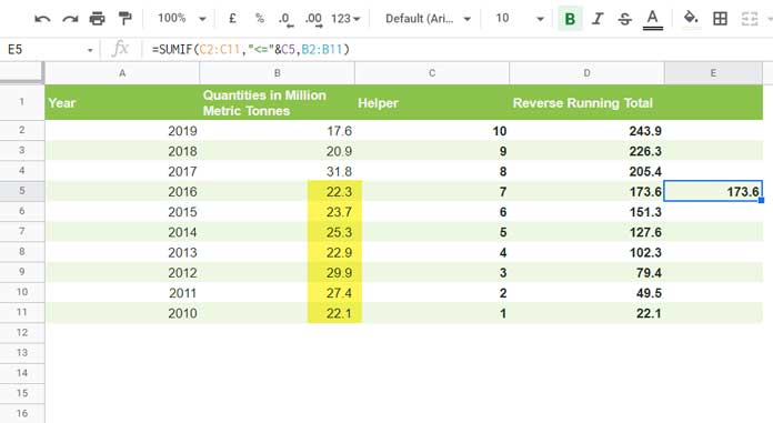
The formula returns the total wheat production in Australia from 2010 to 2016 (highlighted cells).
Because the criterion, i.e., C2:C11<=C5, in column C matches in that highlighted rows.
Resources:
- Running Count in Google Sheets – Formula Examples.
- How to Calculate Running Balance in Google Sheets.
- Array Formula for Conditional Running Total in Google Sheets.
- Sum, Count, Cumulative Sum Comma Separated Values in Google Sheets.
- Cumulative Count of Distinct Values in Google Sheets (How-To).
- Cumulative Balance against Each Payment in Google Sheets.