


In this tutorial, let’s learn how to use alternatives to tilde, asterisk, and question mark wildcards in Sumproduct in Google Sheets.
At present, Google Sheets doesn’t offer support to wildcards in the Sumproduct function. The alternatives are the use of the functions Find/Search or Regexmatch within Sumproduct.
I would stick with Regexmatch. The reason is, it can replace tilde, asterisk, and question mark wildcard characters in Sumproduct, whereas the Search or Find can only use for partial match.
In my opinion, in most of the cases, we can replace Sumproduct formulas with other functions such as Sumif, Countif, Query, etc., in Google Sheets. Still, many Google Sheets users switched from Excel to Google Sheets, prefer Sumproduct.
The reason might be the array support of the said function in Excel.
As far as I know, Google Sheets offers more flexibility in array use though Excel is catching up lately. But there are exceptions too.
Here is one example – Subtotal Function With Conditions in Excel and Google Sheets.
Google has recently improved the capability of the Unique function. Who knows, in the future, Google will improve the Sumproduct too.
Must Check: How to Use SUMPRODUCT Function in Google Sheets.
The Use of Wildcards Asterisk, Question and Tilde in Sumproduct in Google Sheets
If your only purpose of the wildcards uses in Sumproduct is a partial match (alternative to asterisk wildcards on both sides of a criterion like *TV*), you can use Search or Find functions.
The Search isn’t case-sensitive, whereas the Find is case-sensitive. Additionally, you may want to use Isnumber with both of these functions. I’ll come to that in the example part below.
The Regexmatch is the better option as it can handle all three wildcards in the Sumproduct function in Google Sheets.
Let’s start with an example of the use of Search and Isnumber in Sumproduct in Google Sheets.
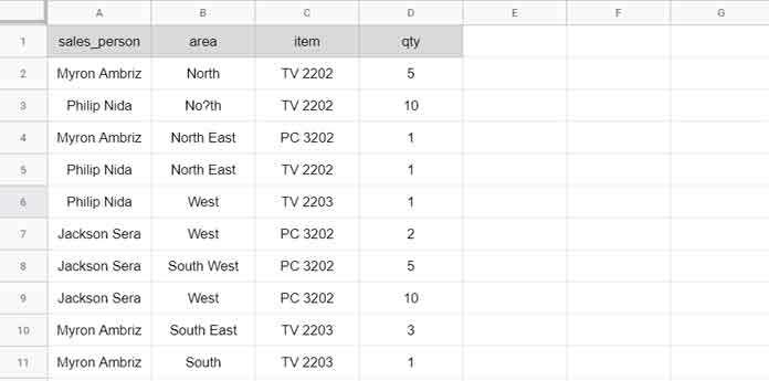
Sample Data (Sheet link included at the last part):
Basic Use with Search or Find Function
Example:
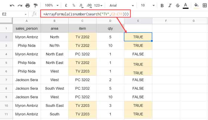
I want to sum the “qty” column if “item” is “TV”. That means I want to use the criterion *TV*.
We can use the following formula for that.
=SUMPRODUCT(isnumber(search("TV",C2:C11)),D2:D11)Formula Explanation
There are two arrays within this formula.
array 1: isnumber(search("TV",C2:C11))
array 2: D2:D11
Syntax: SUMPRODUCT(array1, [array2, …])
The Search formula in “array 1” returns 1 (or the first position of the string TV) in rows wherever it partially/fully matches the string TV.
The Isnumber converts the returned number to TRUE. Please see the image below.
Make E2:E11 empty, and then try the above “array 1” formula in E2.
It will only work for the current row. You must use it as =ArrayFormula(isnumber(search("TV",C2:C11))). But within Sumproduct, the ArrayFormula function is not required.
We require Isnumber because of the following two reasons.
- If the position of the criterion TV is not at the beginning, the Isnumber may return a number other than 1. So you will get the wrong sum of column D. What the formula returns would be the product.
- If there is no match, in such rows, the Search may return #VALUE! So Sumproduct may also return the same error.
Wildcards Using Regexmatch in Sumproduct In Google Sheets
Let’s use the same dataset in cell range A1:D (you will find the sample sheet in the last part of this tutorial).
I am going to write seven formulas. I am sure that those seven formulas will make you learn how to use wildcards in Sumproduct in Google Sheets.
That means you can learn how to replace the following three wildcards with the Regexmatch use in Sumproduct in Google Sheets.
? – used for searching a single character.
* – used for searching multiple characters.
~ – used as a marker to indicate that the next/following character is literal.
Please go through the below table first.
Wildcards to Use in Sumproduct
| Wildcards to Use | Purpose | |
| 1 | TV 220? | Match criterion such as TV 2200, TV 2201, TV 2202, etc. The first six characters must be TV 220 (including the space character). The formula must not be specific about the last character. |
| 2 | TV 22?? | The first five characters must be TV 22. |
| 3 | TV* | Match any string starting with TV. |
| 4 | *TV | Match any string ending with TV. |
| 5 | *TV* | Do a partial match of the string TV. |
| 6 | TV 2*3 | Ignore any number of any characters between 2 and 3. |
| 7 | No~?th | To match the string No?th. |
Here are those seven formula examples to the use of wildcards in Sumproduct in Google Sheets.
Sumproduct Formulas
| Wildcards to Use | Regexmatch in Sumproduct | |
| 1 | TV 220? | =SUMPRODUCT(regexmatch(C2:C11,"^TV 220.$"),D2:D11) |
| 2 | TV 22?? | =SUMPRODUCT(regexmatch(C2:C11,"^TV 22..$"),D2:D11) |
| 3 | TV* | =SUMPRODUCT(regexmatch(C2:C11,"^TV"),D2:D11) |
| 4 | *TV | =SUMPRODUCT(regexmatch(C2:C11,"TV$"),D2:D11) |
| 5 | *TV* | =SUMPRODUCT(regexmatch(C2:C11,"TV"),D2:D11) |
| 6 | TV 2*3 | =SUMPRODUCT(regexmatch(C2:C11,"^TV 2.*3$"),D2:D11) |
| 7 | No~?th | =SUMPRODUCT(regexmatch(B2:B11,"^No\?th$"),D2:D11) |
In the seventh example, the Regexmatch in Sumproduct is not necessary. We can replace that formula with the following one.
=SUMPRODUCT(B2:B11="No?th",D2:D11)Note:- In the above formulas, if you try to use the “Array 1” outside Sumproduct, include the function ArrayFormula.
That’s all about how to use wildcards in the Sumproduct function in Google Sheets.
Thanks for the stay. Enjoy!
Resources: