


Future sheets mean the new sheets you will add to an existing workbook. To include such future sheets in formulas, you must follow a workaround in Google Sheets.
I know some of you may think about using INDIRECT for this. It’s like entering the sheet names as a list and using it as the reference in this function.
Until recently, Google Sheets hadn’t supported this.
Things changed so much in 2022-2023 because of the introduction of a few new functions in Google Sheets, mainly the LAMBDA LHFs.
Understanding the Problem:
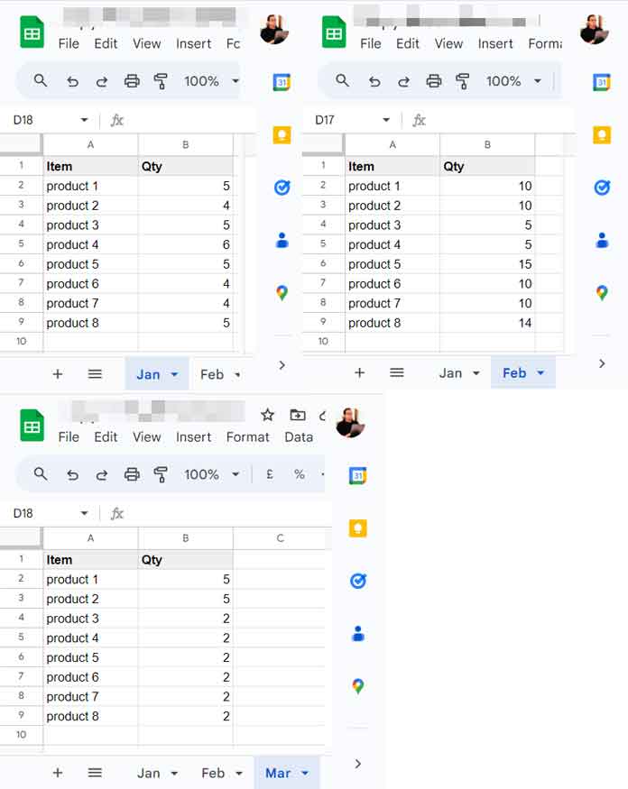
I have three sheets in a workbook with the names “Jan,” “Feb,” and “Mar.” I’ll add a fourth sheet named “Apr” in the future.
We will see how to include that future sheet together with other sheets in SUMIF, QUERY, and COUNTIF formulas.
That will give you a general idea about applying the same technique in other functions.
Sample Data:
Non-Dynamic Way (Hardcoding the Range)
We can either hardcode the range reference from multiple sheets within a formula (non-dynamic) or enter them outside of it in a column (dynamic). We will start with the former one.
Include Future Sheets in SUMIF Formula
Syntax: SUMIF(range, criterion, [sum_range])
The function SUMIF doesn’t work with combined range and will return the error “The argument must be a range.”
So try this in a new sheet in the same workbook that contains the “Jan,” “Feb,” and “Mar” sheets.
Enter the following code in cell A1 in that new sheet to get the range (total data). I’ve included the future sheet, i.e., Apr!A2:A, in this formula.
=LET(range,IFERROR(VSTACK(Jan!A2:A,Feb!A2:A,Mar!A2:A,Apr!A2:A)),FILTER(range,range<>""))You can add more sheets. Put a comma after the fourth sheet and enter it. E.g. Jan!A2:A,Feb!A2:A,Mar!A2:A,Apr!A2:A,May!A2:A.
And this is in cell B1 for the sum_range.
=LET(range,IFERROR(VSTACK(Jan!A2:A,Feb!A2:A,Mar!A2:A,Apr!A2:A)),sum_range,IFERROR(VSTACK(Jan!B2:B,Feb!B2:B,Mar!B2:B,Apr!B2:B)),FILTER(sum_range,range<>""))This B1 formula should contain the range (bolded) in the first part and the sum_range (bolded) in the last part. So that we can ensure that both range and sum_range are equal in size.
So when adding more future sheets, add them in both parts.
Now you can apply SUMIF as follows.
=sumif(A1:A,"Product 6",B1:B)It will return the total “Qty” of the item “Product 6” in the “Jan,” “Feb,” and “Mar” sheets.
When you add future sheets in the workbook, name them as specified in the formula so that it will reflect in the result.
Include Future Sheets in QUERY Formula
Unlike SUMIF, the combined range would work in QUERY. So no need for adding an extra sheet when using this function.
We can use the following QUERY in any sheet in the workbook to get the “Product 6” total from all three existing sheets.
=QUERY(VSTACK(Jan!A2:B,Feb!A2:B,Mar!A2:B),"Select sum(Col2) where lower(Col1) ='product 6' label sum(Col2)''",0)Note:- Specify the criterion in lowercase letters since the function is case-sensitive.
In this, I have combined the range A2:B in all three sheets and then summed the second column if the first column contains the string “Product 6”.
Let me show you how to include a future sheet in the just above QUERY formula.
=QUERY(IFERROR(VSTACK(Jan!A2:B,Feb!A2:B,Mar!A2:B,Apr!A2:B,May!A2:B)),"Select sum(Col2) where lower(Col1) ='product 6' label sum(Col2)''",0)I’ve added Apr and May, two future sheets in it. If they exist, the formula will consider them in the aggregations.
Additionally, I’ve used IFERROR around VSTACK to remove any errors due to the non-availability of any sheets specified.
If I had used the conventional Curly Bracket approach to combine ranges, i.e., {Jan!A2:B;Feb!A2:B;Mar!A2:B;Apr!A2:B;May!A2:B}, the formula would have returned an “Array Literal was missing values for one or more rows” error.
Include Future Sheets in COUNTIF Formula
Unlike SUMIF, the COUNTIF function doesn’t have the “Argument must be a range” issue. So you can use COUNTIF similar to QUERY in any sheet as below.
=COUNTIF(IFERROR(VSTACK(Jan!A2:B,Feb!A2:B,Mar!A2:B,Apr!A2:B,May!A2:B)),"Product 6")It will return the “Product 6” count from available sheets and future sheets as and when you add it.
Dynamic Way (Using COPY_TO_MASTER_SHEET Named Function)
In all the above examples, you may require to edit the formula to remove or add sheets.
You can avoid that by specifying the sheet names in a column in a new sheet in the same workbook and using my COPY_TO_MASTER_SHEET named function to get all the data in one place.
For example, enter the sheet names in A2:A and insert the following formula in C2.
=IFERROR(COPY_TO_MASTER_SHEET(A2:A,"A2:B",2))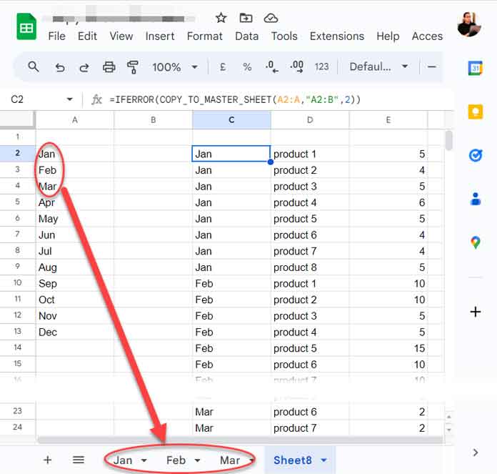
It will combine data from the range A2:B from all the available sheets specified in A2:A.
Use SUMIF, QUERY, COUNTIF, or whatever function you want with this data.
The currently available sheets in the workbook mentioned in the A2:A list are “Jan,” “Feb,” and “Mar.”
When you add the “Apr” sheet to the workbook, the formula won’t include the data from that sheet.
You should copy the C2 formula, delete it from C2, and paste it again. It will refresh the formula.
It applies to all the future sheets you will add to the workbook (not in the list).
There are two options to overcome this copy-paste interaction.
- Only include available sheets in the list. Add a sheet to the workbook first, then enter its name in the list.
- Add all the future sheets to the workbook. You can leave those sheets blank and also hide them.
How do I get this function?
Please check my Named Function guide. You will find a list of named functions including COPY_TO_MASTER_SHEET at the bottom of it.