With the help of a Vlookup Array Formula, you can lookup latest dates in Google Sheets.

Suppose in a column I have a list of different items and the items may repeat many times based on their availability dates.

In a second column, I’ve filled the different availability of each item. As I’ve mentioned, each item has multiple availability dates. So I want to list out the items with latest delivery dates.

The Main function that I’m going to use here is Vlookup. But in the Vlookup we should replace the lookup range, I mean the data rage, with a virtual data range. This virtual data range is the output of SORT and SORTN combination formula.

Example:

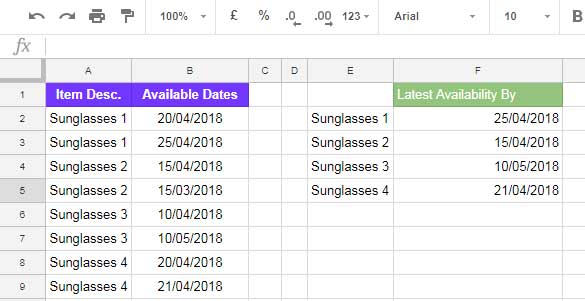
Suppose I have ordered Sunglasses of different brands and it’s in Column A of my spreadsheet.

In Column B, I’ve updated the availability dates of these products. Each item has multiple availability dates and I want to lookup latest available dates of each item.

How to Lookup latest dates in Google Sheets?

What we want to do is lookup column A for Sunglasses and return the latest availability dates from Column B.

How to Lookup Latest Dates in Google Sheets

Steps:

Here are the tips to lookup latest dates in Google Sheets.

1. First sort the column B in descending order. So the items with the latest dates will be on top. No doubt, we can use the function SORT here.

2. Remove all the second, third or multiple occurrences of each item. So the items with the latest dates will be only left. The suitable function here is SORTN.

3. Finally, we can use the result of the second formula as lookup range in Vlookup.

Hope you have got some idea and the logic. Now here is that formula to lookup latest dates in Google Sheets. Please enter this formula in cell F2.

Array Formula to Lookup Latest Dates in Google Sheets

=ArrayFormula(VLOOKUP(E2:E5,SORTN(SORT(A2:B9,2,FALSE,1,TRUE),20,2,1,TRUE),2,FALSE))

Formula Explanation

First, let me begin with the role of SORT (in the Red color font) in this formula. The below is the output of SORT.

We can take only one item from this as an example.

See the item Sunglasses 1 and its available dates. After the sorting in descending order, the latest dated one is on the top. It’s applicable to all items.

Now if we can remove the second occurrences of all the items, the balance available items are the items with the latest dates. We can use SORTN for this purpose.

In the above formula, I’ve highlighted the SORTN with light Yellow color. The output of the SORTN formula would be as below.

SORTN removed all the duplicates and now the only data left is the items with latest available dates.

Must Check: Pick SORTN from my Google Sheets Function Guide

Actually, in most of the cases, this data is enough. But if you want you can use Vlookup to lookup items with the latest dates.

In column E, you can see the lookup values. At present, I’ve put all the items in there. You can limit it to only one item, two items or all the items that you want to look up. The formula and the formula range will remain the same.

Conclusion

With the above tips, you can lookup latest dates in Google Sheets. To lookup earliest dates, I’ve another tutorial on that. Actually the only changes there is in the SORT order.

Similar Topic: Lookup Earliest Dates in Google Sheets in a List of Items

In the real sense, on contrary to my statement in the first para, SORTN is the soul of this formula, not Vlookup.

Of course, Vlookup is a must for lookup dates. But without SORTN Vlookup may not be able to lookup earliest dates.