The WRAPCOLS function lets you quickly turn a single column into multiple columns of a set size. It’s a great trick for dashboards or reports when you want to show more data side by side instead of scrolling down.

But what if you want to insert blank columns between each group to make the layout more readable?

That’s exactly what we’ll cover in this post — how to create WRAPCOLS spaced columns in Google Sheets using a dynamic formula that works even when your data changes.

Basic Use – Wrap a Column into Multiple Columns

Let’s start simple.

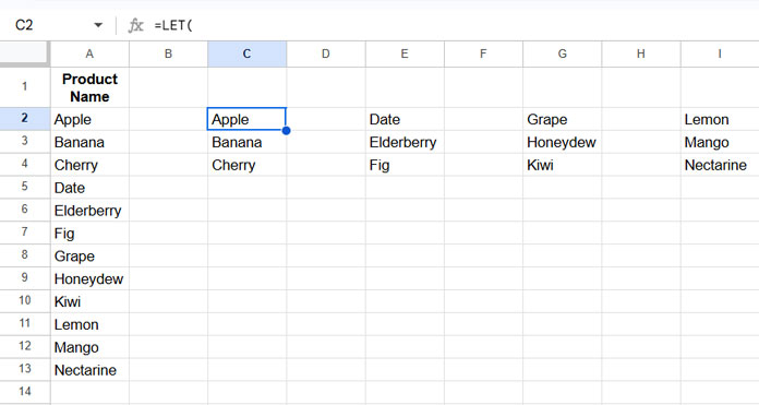
Here’s a list of products in column A:

Product Name
Apple
Banana
Cherry
Date
Elderberry
Fig
Grape
Honeydew
Kiwi
Lemon
Mango
Nectarine

If you want to split this list into columns with 3 rows each, you can use:

=WRAPCOLS(A2:A13, 3)

This gives you:

Handling Blank Values in Open Ranges

If your range is open-ended like A2:A, and might include blanks, use TOCOL to filter out empty cells:

=WRAPCOLS(TOCOL(A2:A, 1), 3)

How to Add Spacing Between Columns with WRAPCOLS

Now, let’s say you want to add some breathing room — like inserting one blank column between each group.

We’ll use a combination of WRAPCOLS, TOCOL, VSTACK, and LET to make this work. Don’t worry, the formula might look a bit complex at first, but the logic is simple.

Generic Formula:

=LET(
  data, IFNA(WRAPCOLS(column, n)),
  data_, VSTACK(data, WRAPCOLS(, n * gap)),
  IFNA(WRAPCOLS(TOCOL(data_, , TRUE), n))
)

Just replace:

• column with your data range (like A2:A13 or TOCOL(A2:A, 1))
• n with the number of rows per group
• gap with the number of empty columns you want between each group

Example: WRAPCOLS Spaced Columns with One Empty Column

Here’s the formula using our product list:

=LET(
  data, IFNA(WRAPCOLS(A2:A13, 3)),
  data_, VSTACK(data, WRAPCOLS(, 3 * 1)),
  IFNA(WRAPCOLS(TOCOL(data_, , TRUE), 3))
)

• n = 3 (rows per column)
• gap = 1 (one blank column between each group)

Result:

Want two blank columns instead? Just update gap to 2:

=LET(
  data, IFNA(WRAPCOLS(A2:A13, 3)),
  data_, VSTACK(data, WRAPCOLS(, 3 * 2)),
  IFNA(WRAPCOLS(TOCOL(data_, , TRUE), 3))
)

How the Formula Works

Let’s break it down:

1. WRAPCOLS(A2:A13, 3) — Wraps the product list into columns with 3 rows each.
2. VSTACK(...) — Adds empty rows below each group based on your gap. For gap = 1, it adds 3 empty rows.
3. TOCOL(..., TRUE) — Turns everything back into a single column (column by column).
4. WRAPCOLS(..., 3) — Re-wraps it again to give you the spaced layout.

It’s a clever layering of wrap, pad, and wrap again — giving you clean blank columns between each data group.

Final Thoughts on WRAPCOLS Spaced Columns in Google Sheets

This method gives you a flexible way to insert empty columns between WRAPCOLS groups without manually editing your layout. It’s especially useful for clean, organized views in dashboards, reports, or printable layouts.

If you ever wanted to fine-tune the way your data looks in Google Sheets, this is a great trick to have in your toolbox.

FAQ – WRAPCOLS Spaced Columns in Google Sheets

1. Can I enter values in the inserted blank columns?

No — if you’re using the formula method, the entire output is formula-generated. That means you can’t manually enter data in those blank columns or any part of the result.

If you want to make changes, you can:

• Copy the entire result (including blank columns)
• Right-click → Paste special → Paste values only

This will turn the formula output into static data that you can edit freely.

2. Can I omit certain values from the spaced-out columns?

Yes! You can filter the original data before passing it to WRAPCOLS using FILTER. For example:

=FILTER(A2:A, A2:A<>"Apple")

This removes specific values (like “Apple”) from the input range. You can also use this inside the spaced-out WRAPCOLS formula to create a clean layout without the unwanted entries.

3. Can I make the number of columns or spacing dynamic?

Yes, you can! Just reference the column height (n) and spacing (gap) from cells instead of hardcoding numbers.

If you put:

• 3 in cell E1 for column height
• 1 in cell F1 for the number of empty columns

Then use:

=LET(
  n, E1,
  gap, F1,
  data, IFNA(WRAPCOLS(A2:A13, n)),
  data_, VSTACK(data, WRAPCOLS(, n * gap)),
  IFNA(WRAPCOLS(TOCOL(data_, , TRUE), n))
)

This way, your layout adjusts automatically when you change the input values — perfect for dashboards or templates.

Related Tutorials

• How to Insert Blank Columns in Google Sheets QUERY
• Find the Last Non-Empty Column in a Row
• Dynamically Remove Last Empty Rows and Columns in Sheets
• Get the Last Column from a Range in Google Sheets
• Filter Out Blank Columns in Google Sheets Using Query Formula