At the time of writing, there’s no TRIMRANGE function in Google Sheets. Sure, we have a function called ARRAY_CONSTRAIN that can trim a range, but it’s not dynamic—you have to manually specify how many rows and columns to return.
So how do you dynamically remove the last (trailing) empty rows and columns from a range? You can use the following formula in Google Sheets:
=LET(
  range, array_or_range,
  ARRAY_CONSTRAIN(
    range,
    MAX(BYCOL(range, LAMBDA(col, ArrayFormula(XLOOKUP("*?", col&"", SEQUENCE(ROWS(col)), , 2, -1))))),
    MAX(BYROW(range, LAMBDA(row, ArrayFormula(XLOOKUP("*?", row&"", SEQUENCE(1, COLUMNS(row)), , 2, -1)))))
  )
)
Here, range refers to the data range or formula result you want to trim.
Just replace 'array_or_range' with your actual range or array formula. The rest of the formula will dynamically calculate the number of rows and columns to retain—cutting off the trailing blanks.
Why Remove Trailing Empty Rows and Columns?
When using open-ended ranges in functions like FILTER, SORT, QUERY, or IMPORTRANGE, you might end up with extra empty rows or columns at the end.
This can be problematic. For example, if you enter any data in an empty column next to the result range, the formula might break—because that empty column is technically part of the result.
So, trimming out those last empty rows and columns dynamically is a smart and practical fix.
Example 1: Dynamically Remove Last Empty Rows and Columns from a Physical Range
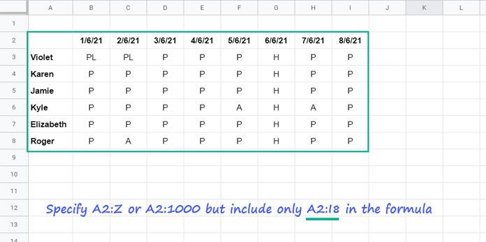
Suppose you want to trim the range A2:Z in Sheet1 from another sheet (Sheet2) using a formula. You can use:
=LET(
  range, Sheet1!A2:Z,
  ARRAY_CONSTRAIN(
    range,
    MAX(BYCOL(range, LAMBDA(col, ArrayFormula(XLOOKUP("*?", col&"", SEQUENCE(ROWS(col)), , 2, -1))))),
    MAX(BYROW(range, LAMBDA(row, ArrayFormula(XLOOKUP("*?", row&"", SEQUENCE(1, COLUMNS(row)), , 2, -1)))))
  )
)
Let’s say your sample data is in A2:I8. This formula will dynamically remove trailing blanks—no manual trimming needed.
Example 2: Dynamically Remove Last Empty Rows and Columns from an Expression
Say you’re importing data using this IMPORTRANGE formula:
=IMPORTRANGE("https://docs.google.com/spreadsheets/d/1BT6Rhtme1j1E2uMVdZP3skC5_N2U5LOg_tmSYVy6Pd8/edit?gid=345964233", "Sheet1!A2:Z")To dynamically remove the last empty rows and columns from the result, simply wrap it with our custom trimming formula:
=LET(
  range, IMPORTRANGE("https://docs.google.com/spreadsheets/d/1BT6Rhtme1j1E2uMVdZP3skC5_N2U5LOg_tmSYVy6Pd8/edit?gid=345964233", "Sheet1!A2:Z"),
  ARRAY_CONSTRAIN(
    range,
    MAX(BYCOL(range, LAMBDA(col, ArrayFormula(XLOOKUP("*?", col&"", SEQUENCE(ROWS(col)), , 2, -1))))),
    MAX(BYROW(range, LAMBDA(row, ArrayFormula(XLOOKUP("*?", row&"", SEQUENCE(1, COLUMNS(row)), , 2, -1)))))
  )
)
Formula Breakdown
The two custom unnamed LAMBDA functions are the core of this formula. One finds the last non-empty row number, and the other finds the last non-empty column number.
Then, ARRAY_CONSTRAIN trims the range based on those values.
Key Parts:
MAX(BYCOL(...)): Returns the last row number that contains a value.MAX(BYROW(...)): Returns the last column number that contains a value.
Syntax Reminder – ARRAY_CONSTRAIN
ARRAY_CONSTRAIN(input_range, num_rows, num_cols)input_range: The actual range or array expression you want to trim.num_rows: Dynamically calculated number of non-empty rows.num_cols: Dynamically calculated number of non-empty columns.
Final Thoughts
This is a solid solution if you’re looking to dynamically remove last empty rows and columns in Google Sheets—whether it’s from a physical range or an expression like IMPORTRANGE. It saves time and makes your formulas more resilient.
Related Resources
- Google Sheets: How to Return First Non-blank Value in a Row or Column
- How to Find the Last Non-Empty Column in a Row in Google Sheets
- VLOOKUP to Get the Last Non-blank Value in a Row in Google Sheets
- Count From First Non-Blank Cell to Last Non-Blank Cell in a Row in Google Sheets
- Get the Header of the Last Non-blank Cell in a Row in Google Sheets
- XMATCH First or Last Non-Blank Cell in Google Sheets
- Get the Headers of the First Non-blank Cell in Each Row in Google Sheets – Array Formula
- Find the Address of the Last Used Cell in Google Sheets


