To dynamically get the last column from a data range in Google Sheets, here’s one efficient and lightweight formula I recommend. I call it “great” for two reasons:

1. It doesn’t rely on resource-heavy functions like QUERY, REGEX, LAMBDA, or Apps Script.
2. The last column doesn’t need to be completely filled. As long as there’s any value in any row, that column will be detected—something traditional methods often miss.

Most formulas you’ll find online use MATCH or XMATCH based on the header row to identify the last column. But that approach fails when the header is empty.

Excel Has TRIMRANGE. What About Google Sheets?

In Excel, there’s a new function called TRIMRANGE that removes trailing empty rows or columns. You can pair it with CHOOSECOLS to get the last column like this:

=CHOOSECOLS(TRIMRANGE(A1:L8), -1)

Unfortunately, TRIMRANGE isn’t available in Google Sheets (at least, not yet). That’s where my method comes in. It performs the same task without any performance hit and is fully dynamic, thanks to the use of the LET function.

All you need to do is specify the range. The formula will return the last non-empty column from that range.

Why Get the Last Column from a Data Range in Google Sheets?

When your dataset grows horizontally over time, you may want to extract the last column dynamically. Here are a few common use cases:

• To chart the first column (like item descriptions) against the last column (latest values).
• To view or calculate with the most recent data in an ever-expanding range.
• To use the last column as a dynamic input in array formulas.

This setup is common when you’re recording data daily, weekly, monthly, quarterly, or yearly—with each time interval in a separate column.

Formula: Get the Last Column from a Range in Google Sheets

=ArrayFormula(
   LET(
      range, A1:E100, 
      bt, NOT(ISBLANK(range)), 
      errv, IF(bt, bt, NA()), 
      rseq, SEQUENCE(COLUMNS(errv), 1, -1, -1), 
      swap, CHOOSECOLS(errv, rseq), 
      row_, SORTN(swap), 
      id, -XMATCH(TRUE, row_), 
      CHOOSECOLS(range, id)
   )
)

This formula will extract the last non-empty column from the range A1:E100.

You can safely replace A1:E100 with any range—even large or partially empty ranges like A1:Z1000. The formula will still return the last used column from that range.

Just make sure the formula is placed outside the data range to avoid circular references.

Example

Here’s a real example using the range C2:I8:

=ArrayFormula(
   LET(
      range, C2:I8, 
      bt, NOT(ISBLANK(range)), 
      errv, IF(bt, bt, NA()), 
      rseq, SEQUENCE(COLUMNS(errv), 1, -1, -1), 
      swap, CHOOSECOLS(errv, rseq), 
      row_, SORTN(swap), 
      id, -XMATCH(TRUE, row_), 
      CHOOSECOLS(range, id)
   )
)

Formula Breakdown

Let’s break this down step-by-step:

• range: Defines the data range to inspect (e.g., C2:I8).
• bt: Returns a boolean array where non-blank cells are TRUE.

• errv: Converts all FALSE values to #N/A using IF(bt, bt, NA()).
• rseq: Generates a reverse column index with SEQUENCE.
• swap: Reverses the column order using CHOOSECOLS and rseq.

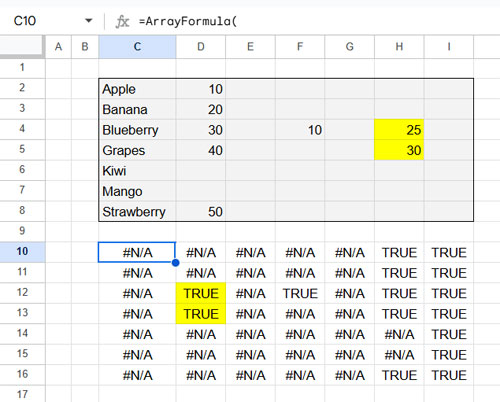
This reversed matrix helps the formula identify the first non-error column from the left, which corresponds to the last used column in the original range.

• row_: Uses SORTN to return a row with at least one TRUE.

{#N/A, TRUE, #N/A, TRUE, #N/A, TRUE, TRUE}

• id: XMATCH returns the position of the first TRUE (non-blank) column in the reversed array. This corresponds to the last used column in the original range. We negate it to use with CHOOSECOLS.
• CHOOSECOLS(range, id): Extracts the last used column.

Combine the First Column and the Dynamic Last Column

As mentioned earlier, one practical use case is to chart the first and last columns together.

Here’s how to do that:

=HSTACK(C2:C8, dynamic_last_column_formula)

Replace C2:C8 with your first column, and insert the last-column formula in place of dynamic_last_column_formula.

The number of rows in the first column and last column should be equal in size.

Resources

Explore more tutorials that use similar techniques:

• Google Sheets: Get the Last Row with Any Data Across Multiple Columns
• Get the First or Last Row/Column in a New Google Sheets Table
• How to Find the Last Non-Empty Column in a Row in Google Sheets
• Dynamically Remove Last Empty Rows and Columns in Sheets
• Find the Address of the Last Used Cell in Google Sheets