


")


")

")
")
 in Excel & Google Sheets")


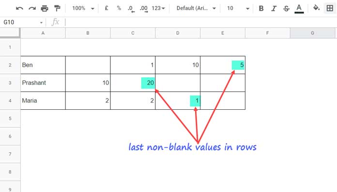
In this tutorial, you’ll learn how to use VLOOKUP to get the last non-blank value or item in the found row in Google Sheets.
How Is This Different from a Regular VLOOKUP Formula in Sheets?
Normally, when using VLOOKUP in Sheets, we specify a column in the lookup range to return the result. In VLOOKUP’s terms, this is called the index (the relative position of the output column).
For example, we can use the following VLOOKUP formula in Google Sheets to search the range A2:E for the name “Maria” in column A and return a value from the second column of the found row:
=VLOOKUP("Maria", A2:E, 2, FALSE)In this example, the index number (the column position for the result) is 2, so we will get the value from cell B4.
Syntax: VLOOKUP(search_key, range, index, [is_sorted])
VLOOKUP Formula to Get the Last Non-blank Value in the Found Row
Here’s a generic formula to find the last non-blank value in the found row:
=CHOOSECOLS(TOROW(ARRAYFORMULA(VLOOKUP(search_key, range, SEQUENCE(1, COLUMNS(range)), FALSE)), 3), -1)Where:
- search_key is the value you’re looking up.
- range is the lookup range where VLOOKUP searches for the search_key in the first column.
This formula will return the result from the last non-blank column in the row.
Example
Let’s say the sample data is in the range A2:E. To search for “Maria” in column A and return the value from the last non-blank cell in the found row, use the following formula:
=CHOOSECOLS(TOROW(ARRAYFORMULA(VLOOKUP(G2, $A$2:$E, SEQUENCE(1, COLUMNS($A$2:$E)), FALSE)), 3), -1)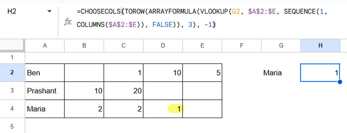
How Does This Formula Work?
ARRAYFORMULA(VLOOKUP(G2, $A$2:$E, SEQUENCE(1, COLUMNS($A$2:$E)), FALSE)): The VLOOKUP searches for “Maria” in the range A2:E and returns the entire row.TOROW(..., 3): This removes empty cells from the returned row.CHOOSECOLS(..., -1): This returns the last non-blank value from the row.
This is how the VLOOKUP formula works to search for a value in a range and return the last non-blank value in the found row.
VLOOKUP to Get the Last Non-blank Value in Each Row in Google Sheets
You can use the above VLOOKUP formula to find the last non-blank value in each row.
In cell F2, enter the following formula and drag it down:
=CHOOSECOLS(TOROW(ARRAYFORMULA(VLOOKUP(A2, $A$2:$E, SEQUENCE(1, COLUMNS($A$2:$E)), FALSE)), 3), -1)The difference here is that we’ve specified the first column letter (A2) as the search key.
Auto-expanding the Formula Using MAP
If you want to auto-expand the formula for an entire column, you can use the MAP function as follows:
=IFERROR(MAP(A2:A, LAMBDA(val, CHOOSECOLS(TOROW(ARRAYFORMULA(VLOOKUP(val, A2:E, SEQUENCE(1, COLUMNS(A2:E)), FALSE)), 3), -1))))The IFERROR function ensures that errors from blank rows are removed.
Resources
- Google Sheets: How to Return First Non-blank Value in a Row or Column
- How to Find the Last Non-Empty Column in a Row in Google Sheets
- How to Dynamically Exclude Last Empty Rows and Columns in Google Sheets
- Count From First Non-Blank Cell to Last Non-Blank Cell in a Row in Google Sheets
- Get the Header of the Last Non-blank Cell in a Row in Google Sheets
- XMATCH First or Last Non-Blank Cell in Google Sheets
- Get the Headers of the First Non-blank Cell in Each Row in Google Sheets – Array Formula
- Find the Address of the Last Used Cell in Google Sheets