With the help of the function Vlookup, we can import matching values from one Spreadsheet to another in Google Sheets. Let me detail how to Vlookup Importrange in Google Sheets.
If you know about using Vlookup and Importrange functions, then Vlookup+Importrange is just child’s play.
Many Google Spreadsheets users doubt they may use Vlookup+Importrange or Query+Importrange to conditionally import data between two Google Sheets files.
The answer is you can use both. But there is some difference, and I’ll explain that below.
So this is an advanced tutorial that covers not only the use of Vlookup in Importrange but also how to use Query in Importrange in Google Sheets.
I know you are not new to Vlookup or Importrange, and that’s why you are here to learn how to use Vlookup in Importrange in Google Docs Sheets.
Still, if you think it’s time to brush up on your Vlookup/Importrange skills, please check my Google Sheets Functions guide.
I am explaining the below Vlookup and Importrange tips in this post.
- How to use Vlookup with Importrange Function in Google Sheets?
- How to Use Multiple Conditions in Vloookup in Importrange Data in Google Sheets?
Then the following Query function usage with Importrange.
- How to Use Query with Importrange for Importing Matching Values?
Here we go!
How to Vlookup Importrange in Google Sheets
For this example, I am using two Google Sheets files. Even though the file names are unimportant, please note them for your reference.
File 1 (Workbook 1): Sales.
File 2 (Workbook 2): Analysis.
We will import data from the first Google Sheets file, i.e., “Sales,” to the second Google Sheets file, i.e., “Analysis.”
That means I will use the Vlookup+Importrange combination formulas in the file “Analysis.”
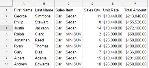
Here is the sample data in the “Sales” file. The data range is A1:F, and the sheet name (worksheet name) is “Sheet1.”
Formula Examples to the Use of Vlookup with Importrange Function in Google Sheets
I am in the Sheet “Analysis.”
Let me show you from within this Sheet how to search Sheet1!A1:F in the “Sales” file and return values.
Basic Example of How to Vlookup Importrange in Google Sheets
In the file “Analysis,” I have the search key (first name) “Justin” in cell A2.
I want to Vlookup this name in A2:A in Sheet1 in the “Sale” file and return the corresponding value from column F.
Steps
The thumb rule is the Vlookup function searches down the first column of a table for the search key. So we must import the table starting from that column.
1. First, Open the “Sales” workbook and grab the Spreadsheet URL from the address bar. You must ensure that the active tab is “Sheet1,” which contains the data to lookup.
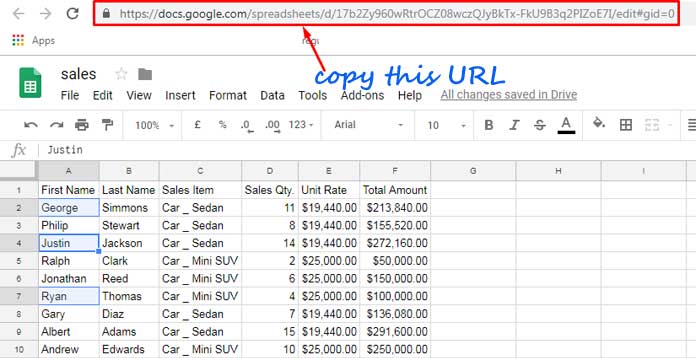
2. Go to the file “Analysis” and insert the following Importrange formula in cell B1.
=IMPORTRANGE("URL","Sheet1!A1:F")Syntax: IMPORTRANGE(spreadsheet_url, range_string)
3. Replace the text “URL” with the copied Spreadsheet URL.
4. If it returns a #REF error, hover over it and “Allow access”. This helps import data from a source sheet (Sales) to a destination sheet (Analysis).
5. Wrap it with the Vlookup function as below.
=VLOOKUP(A2,IMPORTRANGE("URL","Sheet1!A1:F"),6,FALSE)Syntax: VLOOKUP(search_key, range, index, [is_sorted])
This Vlookup Importrange formula would return the value 272160.00 from the return column specified in Vlookup, i.e., 6.
Anatomy of the Vlookup Formula
search_key: A2
Cell reference A2 in the “Analysis” (destination file) contains the search key, which is the name “Justin.”
range: IMPORTRANGE(“URL”,”Sheet1!A1:F”)
The lookup range, the second parameter in the formula, is in another file, which is “Sales.”
index: 6
The index here is column number 6 (column F), from which the Vlookup returns the value.
is_sorted: FALSE
It ensures an exact match of the search key in the first column of the table.
Vlookup Importrange with Multiple Search Keys in the Same Column
Note:- I recommend you to check this tutorial, Vlookup Array use, before proceeding further – How to Use Vlookup to Return An Array Result in Google Sheets.
Vlookup+Importrange supports almost all the Advanced Vlookup flavors.
But the formula may seem complex due to replacing of Vlookup range with the Importrange.
Let’s use Vlookup in Importrange with multiple search values.
In the “Analysis” file, I have the following search keys in the range A2:A4.
Justin
Andrew
Jonathan
Here is the Vlookup Importrange combination formula in Google Sheets with multiple search keys in the same column.
=ARRAYFORMULA(IFERROR(VLOOKUP(A2:A,IMPORTRANGE("URL","Sheet1!A1:F"),6,0)))Can you point out how this formula differs from our earlier formula?
This Vlookup is an Array Formula. That means we expect an array result from Vlookup.
Since Vlookup is not an Array Formula, made it an array formula by wrapping it with the function ArrayFormula.
Further, since the search keys are in A2:A4, used A2: A (infinite range to include future search keys).
Included the IFERROR to avoid #N/A error.

Multiple Conditions/Criteria in Different Columns in Vlookup+Importrange Formula
This formula may be confusing to many users compared to the above two.

So I highly recommend you refer to this guide – How to Use VLOOKUP with Multiple Criteria in Google Sheets. Here in this tutorial, there is only a slight variation.
In regular use, the Vlookup searches down the first column in a range.
In multiple criteria Vlookup, the formula search downs two columns (you can include more columns, though). Again we want to do it in an imported range.
Let’s see How to Vlookup the first column + another column in Vlookup Importrange.
This time, I want to search down the search keys in columns A and B in the imported range, which means the first name and last name.
Search Keys (A2:B4):
Justin | Jackson
Andrew | Edwards
Jonathan | Reed
Formula:
=ARRAYFORMULA(VLOOKUP(A2:A&B2:B,{IMPORTRANGE("URL","Sheet1!A2:A")&IMPORTRANGE("URL","Sheet1!B2:B"),IMPORTRANGE("URL","Sheet1!C2:F")},5,FALSE))You must replace all three URLs in the formula with the “Sales” URL.
The logic in this formula is like this:
- Join, combine, or concatenate the search keys using the ampersand sign.
- Join the related columns in the Vlookup range using the ampersand sign.
- Earlier, the output column was the 6th column in the lookup table. Now we have only five columns because of combining two columns in the range. So use column index number 5 instead of 6.
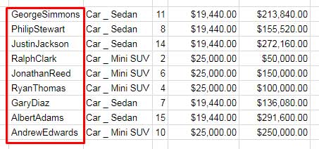
Didn’t get it? See this new combined range returned by multiple Importrange formulas and ampersands.
Performance Enhancement Using LET
One of the issues of using multiple importrange is it affects the performance. It can slow down the calculation.
The new LET function sorts out this issue. We can rewrite the above formula as below.
=ARRAYFORMULA(LET(sk,A2:A&B2:B,rg,IMPORTRANGE("URL","Sheet1!A2:F"),VLOOKUP(sk,{CHOOSECOLS(rg,1)&CHOOSECOLS(rg,2),CHOOSECOLS(rg,{3,4,5,6})},5,0)))LET Syntax: LET(name1, value_expression1, [name2, …], [value_expression2, …], formula_expression)
name1: sk
value_expression: A2:A&B2:B
name2: rg
value_expression2: IMPORTRANGE("URL","Sheet1!A2:F")
The sk is the name of the Vlookup search keys, and rg is the name of the Importrange formula (Vlookup range).
formula_expression: VLOOKUP(sk,{CHOOSECOLS(rg,1)&CHOOSECOLS(rg,2),CHOOSECOLS(rg,{3,4,5,6})},5,0)
I’ve used the Vlookup in the formula expression part. The CHOOSECOLS is the extract columns from the imported range. Then combined the first two search columns.
In the above Vlookup Importrange example, we used importrange only once.
What interesting is we can use the Importrange function with XLOOKUP to import values.
Xlookup Importrange Alternative:
=ARRAYFORMULA(LET(sk,A2:A&B2:B,rg,IMPORTRANGE("URL","Sheet1!A2:F"),XLOOKUP(sk,CHOOSECOLS(rg,1)&CHOOSECOLS(rg,2),CHOOSECOLS(rg,6))))Syntax: XLOOKUP(search_key, lookup_range, result_range, [missing_value], [match_mode], [search_mode])
We have used the bolded arguments only.
Query as Vlookup + Importrange Alternative in Google Sheets
You can use Query as an alternative to Vlookup. We can use its filter capability to get the required result in a second sheet from the first sheet.
Query with Google Sheets Importrange for Importing Matching Values
Example:
The search key in cell A2 in the “Analysis” file is “Justin.”
The Query can match this value in the Importrange data (“Sales” file data) and return the corresponding value from column 6.
=Query(IMPORTRANGE("URL","Sheet1!A2:F"),"Select Col6 where Col1='"&A2&"'")If you have multiple search keys in Column A, then you must drag this formula down.
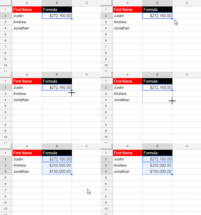
Of course, we can include all the search keys in one go using Matches regular expression match in Query.
Here is another example of the Vlookup Importrange formula alternative in Google Sheets.
This time see how to search ‘down’ two columns using Query.
It is similar to the multiple conditions in the Vlookup Importrange formula.
=QUERY(IMPORTRANGE("URL","Sheet1!A2:F"),"Select Col6 where Col1='"&A2&"' and Col2='"&B2&"'")You may drag it down to include multiple search keys.

Conclusion
The Query in Importrange in Google Sheets scores over the Vlookup Importrange only at one point.
That is the simplicity of the Query to use and understand.
Leaving that aside, Vlookup Importrange is far better as it can quickly populate an array result.
Use the LET function, as per my example, when you want to combine multiple Importrange formulas for Lookup. That’s a performance enhancer.





Hello,
I am trying to use the QUERY + IMPORTRANGE formula.
Here is the formula:
=Query(IMPORTRANGE("1x0O6WEg-itX_0eGChEFhZAnrlN5cRDdvuyyc6rPt__Q", "'Payment Record'!A1:E"),
"Select Col4 where Col2='"&Orders!C8&"' and Col3='"&B2&"'")
Where Orders!C8 is a string from another sheet of the current workbook, and B2 is a date.
The IMPORTRANGE table’s Col2 and Col3 columns are the same data type.
The value it returned was the Col4 header value.
I hope you will be able to assist.
Hi, Khairy,
That’s not the way you should use date criteria in Query.
Replace
Col3='"&B2&"'withCol3=date '"&TEXT(B2,"yyyy-mm-dd")&"'Hi, This is exactly all the pieces of information and experience I was looking for.
I was stuck with
"query(importrange("as I needed an array result, which was impossible.Thank you very much for sharing your knowledge with simples explanations and step decomposition of the formulas.
Hello,
I’m trying to figure out how to import data from another sheet with a condition.
I have used the regular Vlookup + Importrange and it worked beautifully when I didn’t need conditions. But now I want to add to it that I only want the data imported to the new table if on the original table the column D = “September”.
Would you be able to help? I really appreciate it!
Hi, Luiza,
You may read this.
How to Use Query With Importrange in Google Sheets.
If you still have issues, you may create a sample sheet and leave the URL in the comment reply below. I’ll try my best.
Yes, I have the same problem… the reference sheet that I want to import info from is very large … 26 columns and over 30000 rows.
=VLOOKUP(K3,IMPORTRANGE("url","Sheet 1!A:Z"),2,FALSE)and the error message is #ERROR! results too large.
Hope you can assist, Is there a limit on the “range” to be imported with the VLookup.
The range is A9:W7900, I get a #REF! error, if I reduce the range to say, A9:1500 it works fine.
What am I missing?
Hi, Jaime,
Hover your mouse pointer over the (cell containing) error and see the error message. So you will get an idea why the error is happening.
Best,