


")


")

")
")
 in Excel & Google Sheets")


In this tutorial, I’ve included all the essential tips and tricks to help you master the VLOOKUP function in Google Sheets.
You’ll find 10 different variations of the VLOOKUP formula in Google Sheets, explained with practical, real-life examples.
Learn how to use the basic VLOOKUP function with a simple, beginner-friendly example. I’ve written this in a way that even a complete newbie can follow along easily.
Once you’re comfortable with the basics, explore the advanced tips, tricks, and formula variations that make this one of the most versatile functions in Google Sheets.
Function Syntax and Arguments
Syntax
VLOOKUP(search_key, range, index, [is_sorted])Arguments Explained
- search_key: The value (text, number, date, etc.) to search for.
Must be in the first column of the range. - range: The dataset to search through.
Only the first column of this range is searched for the search_key. Tip: If your lookup column isn’t the first, there’s a workaround later in this tutorial. - index: The column number (within the range) from which to return the result.
The first column is 1. - is_sorted(optional):
FALSE(recommended): Looks for an exact match. If not found, it returns#N/A. You can handle this withIFNA.TRUE(default): Searches for the closest match that is less than or equal to the search_key. Use this only if the first column of the range is sorted in ascending order.
Basic Example Formula
VLOOKUP is one of the must-know functions for anyone working with spreadsheets — and I’ve included all the key variations in one place so you can master it with confidence. Let’s start with a simple example to understand the basics.
Purpose of VLOOKUP in Google Sheets
The function searches vertically (i.e., down the first column of a range) for a value and returns a value from another column in the same row.
Let me break it down:
Example:
You want to find the “Test 2” score of “Student 3.”
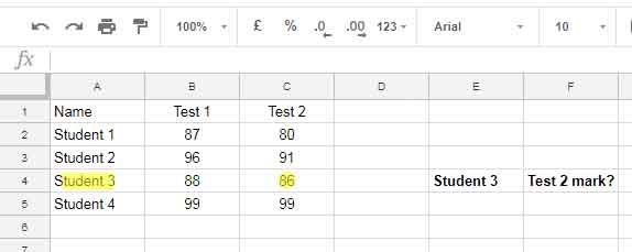
"Student 3"is yoursearch_key- It’s in the first column
- “Test 2” is in column 3 (so index = 3)
=VLOOKUP("Student 3", A2:C5, 3, FALSE)This returns: 86
Key Tip:
Always use FALSE for the fourth argument unless your data is sorted. It ensures you’re getting an exact match.
VLOOKUP Advanced Tips & Formula Variations
1. Search Keys from a Range
Want to look up prices for multiple items like “Apple” and “Mango”? No problem.
=ARRAYFORMULA(VLOOKUP(D2:D3, A2:B5, 2, FALSE))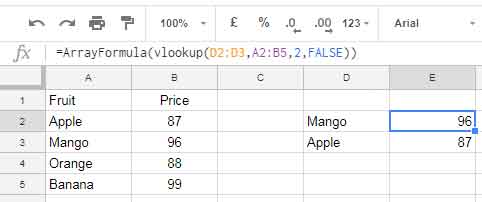
Or, you can hardcode multiple search keys using {}:
=ARRAYFORMULA(VLOOKUP({"Mango"; "Apple"}, A2:B5, 2, FALSE))Related: Retrieve Multiple Values Using VLOOKUP in Google Sheets
2. Return an Entire Row
Yes, you can return an entire row with VLOOKUP.
=ARRAYFORMULA(VLOOKUP("Student 2", A2:D5, {1, 2, 3, 4}, FALSE))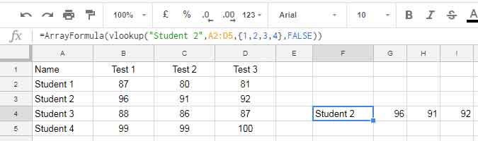
But here’s a more flexible version:
=ARRAYFORMULA(VLOOKUP("Student 2", A2:D5, SEQUENCE(1, COLUMNS(A2:D5)), FALSE))Here, SEQUENCE(1, COLUMNS(A2:D5)) generates a horizontal sequence of numbers matching the number of columns in the range.
This way, the formula automatically adapts—even if you insert or delete columns—without needing to manually update the column numbers.
3. Variable Column Index
Instead of using a fixed number like 4, make the column index dynamic:
=VLOOKUP("Student 2", A2:D5, COLUMNS(A2:D2), FALSE)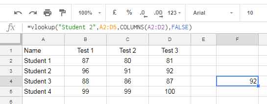
To return the second-to-last column:
=VLOOKUP("Student 2", A2:D5, COLUMNS(A2:D2)-1, FALSE)
Why this works:COLUMNS(A2:D2) returns the number of columns in the range — in this case, 4. So, the third argument in VLOOKUP becomes dynamic.
Why it’s better:
Using COLUMNS() makes your formula more robust against structural changes. For example, if you later insert or delete a column within the range, the formula automatically adjusts. This prevents hardcoded index numbers from breaking when your sheet layout changes.
4. Leftward VLOOKUP (Lookup in a Column to the Right)
By default, VLOOKUP in Google Sheets only searches in the first column of the range.
But here’s a workaround when the search key isn’t in the first column.
Let’s say “Student 3” is in column D.
=VLOOKUP("Student 3", {D2:D5, A2:C5}, 2, FALSE)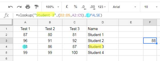
This rearranges the columns virtually—putting D first—so VLOOKUP works as expected.
See also: Reverse VLOOKUP in Google Sheets: Find Data Right to Left
5. Case-Sensitive VLOOKUP
VLOOKUP by default is not case-sensitive.
Suppose:
- A4:
"IL102B" - A5:
"IL102b"
You want to match "IL102b" exactly (case-sensitive). This formula won’t help:
=VLOOKUP("IL102b", A2:G5, 5, FALSE)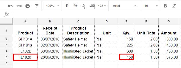
It returns the first match, ignoring case.
Solution:
Use QUERY (which is case-sensitive) to filter the data:
=VLOOKUP("IL102b", QUERY(A2:G5, "SELECT * WHERE A = 'IL102b'"), 5, FALSE)This ensures only the correct-case match is returned.
More here: Case-Sensitive VLOOKUP in Google Sheets
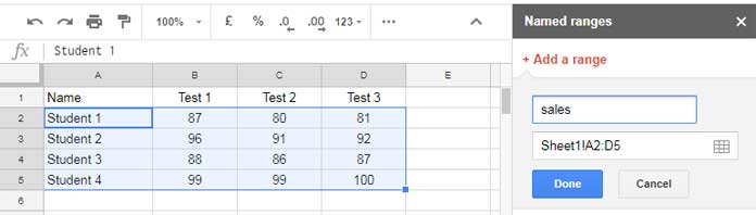
6. Named Ranges
Yes, VLOOKUP in Google Sheets supports named ranges.
Let’s say you named A2:D5 as "sales":
=VLOOKUP("Student 3", sales, 4, FALSE)Cleaner, more readable formulas!
Learn more: Using Named Ranges in VLOOKUP
7. Combine Search Keys (Multiple Conditions)
Want to find the price of “Cement” sold by Vendor “Z”?
- Combine columns A & B (
A2:A7 & B2:B7) - Search for
"CementZ"
=ARRAYFORMULA(VLOOKUP("CementZ", {A2:A7 & B2:B7, C2:C7}, 2, FALSE))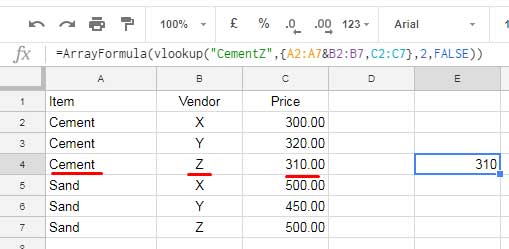
This is the simplest way to simulate multiple conditions in a single VLOOKUP. But there are more advanced (and proper) ways to handle multiple criteria.
More: VLOOKUP with Multiple Criteria in Google Sheets: The Proper Way
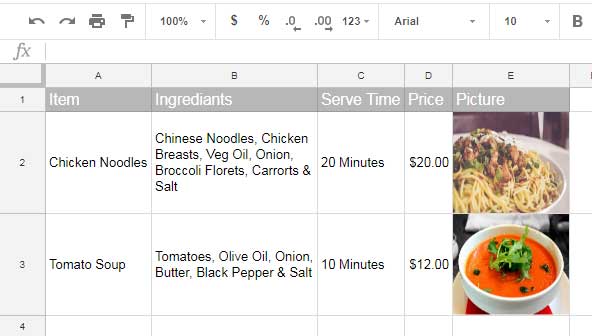
8. Image VLOOKUP
Need to return an image?
=VLOOKUP("Chicken Noodles", A2:E3, 5, FALSE)This will return the image in column E corresponding to the search key in column A.
Helpful links:
9. Wildcard Characters
You can use wildcards like * and ? in VLOOKUP when is_sorted is FALSE.
Example:
=VLOOKUP("Y*", A2:B6, 2, FALSE)Or with a cell reference:
=VLOOKUP(D1 & "*", A2:B6, 2, FALSE)
*: Matches multiple characters?: Matches a single character~: Escape character (e.g.,~*matches a literal asterisk)
10. Table References
With the new Insert → Table feature in Google Sheets, you can create structured tables that support named table references — just like in Excel.
Once you’ve inserted a table (via Insert > Table or by selecting a range and choosing Convert to table), you can refer to it by name in your formulas:
=VLOOKUP("Apple", Table1, 2, FALSE)Here, Table1 is just an example.
You’ll need to use the actual name of your table — which Google Sheets assigns automatically (like Table1, Table2, etc.), or you can rename it from the table properties panel.
This approach keeps your formulas cleaner and ensures they stay updated even if the table grows or changes over time.
Conclusion
If you search this site, you’ll find even more ways to use VLOOKUP in Google Sheets in real-life scenarios.
That’s a wrap on the core techniques! I hope this guide helped you get more confident using VLOOKUP.
Useful VLOOKUP Resources for Google Sheets
Here are more advanced tutorials and use cases involving VLOOKUP in Google Sheets:
- Using VLOOKUP to Find the Nth Occurrence in Google Sheets
- Comparison of VLOOKUP Formula in Excel and Google Sheets
- LOOKUP, VLOOKUP, and HLOOKUP: Key Differences in Google Sheets
- How to Perform Two-Way Lookup Using VLOOKUP in Google Sheets
- Highlight VLOOKUP Results with Conditional Formatting in Sheets
- How to VLOOKUP IMPORTRANGE in Google Sheets (Formula Examples)
- VLOOKUP Skips Hidden Rows in Google Sheets
- Common Errors in VLOOKUP in Google Sheets
- VLOOKUP vs XLOOKUP in Google Sheets: Key Differences & Use Cases
The left-ward Vlookup, this was neat. Thanks for publishing this. All the best in saving the rest of us considerable time and grief, I know it helped me with Google Sheets.