This tutorial explains how to view and edit named ranges in Google Sheets.
What are Named Ranges? Named Ranges involve assigning a name to a group of cells. This allows us to quickly reference them in formulas without needing to use cell addresses.
In this tutorial, I will discuss how to view named ranges in Google Sheets and also how to delete them.
Why is this necessary?
It all begins when you are working on a shared sheet that contains formulas entered by another user and shared with you.
To comprehend the formulas in a shared spreadsheet, it’s essential to first check for the existence of named ranges in that sheet, as the use of named ranges is common among spreadsheet users.
If you are new to our page, there is already a tutorial on adding named ranges in Google Sheets. Please switch to the tutorial below and come back here. This will help you understand the usefulness of this awesome feature.
Related: How to Use Named Ranges In Google Sheets for Cleaner Formulas
Viewing Named Ranges in Google Sheets
There are two ways to view named ranges in Google Sheets, and the first method is solely for observing the range without the ability to edit or delete it.
Method 1:
In the first method, you need to know the name of the range. Enter the named range’s name in a cell, starting with an equal sign.
Example: =PurchaseValue
This will display the named range and the cell range it encompasses. To navigate to that range, follow these steps:
Use the keyboard shortcut Ctrl + G (Mac) to open the “Go to range” dialog. For Windows, press Alt + / and type “Go to” to access the “Go to range” dialog.
Enter the named range name and press Enter. This will take you to the named range.
Method 2:
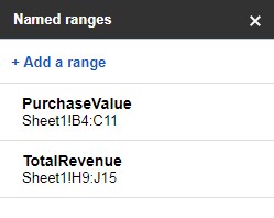
Click on “Data” > “Named ranges” to view the list of named ranges in the sidebar panel.

Simply clicking on a named range in the list will direct you to the covered area (cells). This method allows you to view, edit, and delete named ranges.
How to Delete Named Ranges in Google Sheets
After exploring two methods to view named ranges in Google Sheets, let’s now focus on the process of editing or deleting them.
To edit or delete a named range, follow these steps:
- Navigate to “Data” > “Named ranges.”
- Hover your mouse over the named range that you want to edit or delete. Click on the pencil icon.
- To delete the named range, click on the trash bin icon. If you wish to edit it, simply modify the range in the provided field.
What happens when a formula that uses a deleted named range in Google Sheets?
While the formula might still return the correct result, upon inspection, you will notice that the named range’s name has been replaced by #REF!. It is crucial to correct the formula promptly to prevent potential issues later on.
How to Locate Formulas that Use Deleted Named Ranges in Google Sheets
The most straightforward method to locate a formula that uses a deleted named range involves using conditional formatting (cell highlighting).
Assuming your sheet contains the range A1:Z1000, follow these steps to highlight cells containing formulas that use deleted named ranges:
- Go to “Format” > “Conditional formatting.”
- In the sidebar panel, find “Apply to range.” If you already have existing rules, click “Add another rule” to locate it.
- Enter the range A1:Z1000.
- Under “Format rules,” select “Custom formula is…” and enter the following formula:
=REGEXMATCH(FORMULATEXT(A1), "REF") - Click Done. This will highlight all cells containing formulas with a “REF” error. This method helps identify cells with formulas using deleted named ranges.
Note: If your file has multiple sheets, you may need to apply this method to all sheets. Additionally, be aware that highlighting may impact the performance of your sheet, especially with large volumes of data.
Resources
This tutorial has outlined how to view, edit, and delete named ranges, as well as locate formulas containing deleted named ranges in Google Sheets. Here are some advanced uses of named ranges.
- How to Use Named Ranges in Query in Google Sheets
- The Use of Named Ranges in Sumif in Google Sheets
- The Use of Named Ranges in Vlookup in Google Sheets
- Importrange Named Ranges in Google Sheets
- Dynamic Column Id in Query Importrange Using Named Ranges
- Auto-Expand Named Ranges in Google Sheets to Accommodate New Rows
- Highlighting Named Ranges in Google Sheets
- How to Use Named Ranges in Conditional Formatting in Google Sheets


Thank you for your direction.
Now that I have a good-sized spreadsheet, loaded with many named ranges, I need to obtain a list of those named ranges so that I may print the list for documentation purposes.
Using the display function in Sheets works well, but limits my scanning through them to use the scroll feature to move up and down through the list.
What I really need is a list of these named ranges so that when in the middle of constructing complicated formulas, I can simply consult the one-page hardcopy of the names I would like to include. Excel allows printing them. Can Sheets do the same?
Thank you kindly.
Hi, Gordon McLaughlin,
By using Google Apps Script you may be able to do that. But that’s not my cup of tea 🙁
You may please follow this “StackOverflow” thread:
https://stackoverflow.com/questions/29635264/how-to-process-all-named-ranges-in-a-google-sheet