


 of a dataset excluding some user-specified proportion of data.)
To exclude outliers in the average calculation, use the function TRIMMEAN instead of AVERAGE. The TRIMMEAN function in Google Sheets returns the mean (average) of a dataset excluding some user-specified proportion of data.
The proportion of the dataset in this function can be specified either in percentages like 10%, 50%, etc. or in equivalent numbers like 0.1, 0.5, etc.
The TRIMMEAN will exclude values from high and low ends of the dataset (values much higher than or smaller than most of the values in the dataset) based on this percentage.
Why should we use the TRIMMEAN function instead of the AVERAGE function in Google Sheets? Can you provide one example?
Assume you have a dataset like this in Docs Sheets and want to calculate the average.
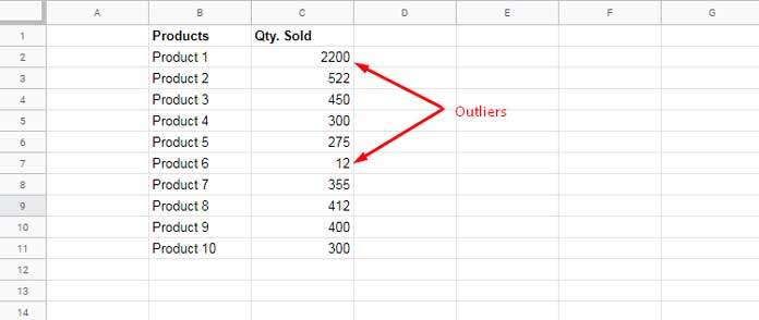
If you use the AVERAGE function the outliers 2200 and 12 will make a huge impact on the average quantity sold. Because these two values lie outside most of the other values in the range C2:C11.
Please do note that the mean (average) is the sum/count. The average sales of the above 10 products are 522.6.
=average(C2:C11)If you remove the outliers, then you will get the average value, i.e. 376.75.
In a smaller dataset or you can say array/range, you can manually exclude the outliers as above, but not possible in a larger dataset. Here comes the use of TRIMMEAN in Google Sheets.
TRIMMEAN – Syntax and Arguments
Syntax:
TRIMMEAN(data, exclude_proportion)Arguments:
data – The range/array containing the dataset to consider.
exclude_proportion – The proportion of the dataset to exclude from the top and tail (or you can say to exclude from the extremities of the set).
This proportion must be greater than or equal to 0 (or 0%) and less than 1 (or 100%). When specifying the proportion in the TRIMMEAN function please keep remembering this.
Smaller the data size, larger the proportion
Example Formula:
=TRIMMEAN(C2:C11,0.2)
or
=TRIMMEAN(C2:C11,20%)
Result: 376.75
The TRIMMEAN formula excludes the outliers 2200 and 12 from the average calculation.
Conditional TRIMMEAN in Google Sheets
For conditional TRIMMEAN in Google Sheets, you can use the FILTER function to filter the ‘data’. You can also use Query instead of FILTER.
Here is one example of conditional TRIMMEAN in Google Sheets. To further deepen the use of condition, do master the Filter function.
Must Check: Google Sheets Function Guide.
=trimmean(filter(C2:C11,B2:B11<>"Product 1"),10%)This Google Sheets TRIMMEAN is an example of conditional average calculation excluding outliers.
=trimmean(query(B2:C11,"Select C where B <>'Product 1'"),10%)The above formulas find the TRIMMEAN excluding the product “Product 1” from the dataset. That means I have used one criterion in the calculation.
If you know the use of the above two data manipulation functions (Query and Filter), then you can include more conditions easily in the average calculations excluding outliers.
Related Reading: