Find Top 10 Unique Names by Score in Google Sheets

In several scenarios, you might need to find the top 10 unique names by the score in Google Sheets. This is commonly used in sports rankings, gaming leaderboards, and academic competitions where multiple attempts exist. The goal is to ensure that each participant appears only once, with their highest score considered.

You can achieve this using either a combination of SORT and SORTN or the QUERY function.

How to Find the Top 10 Unique Names by Score in Google Sheets

Formula Option 1: Using SORT and SORTN

=SORT(SORTN(SORT(A2:B, 2, FALSE), 10, 2, 1, TRUE), 2, FALSE)

Formula Option 2: Using QUERY

=QUERY(A2:B, "select Col1, max(Col2) group by Col1 order by max(Col2) desc limit 10 label max(Col2)''")

When using these formulas, replace A2:B with your actual data range, where column A contains names and column B contains scores.

Google Sheets Example: Find Top 10 Unique Names by Score

Sample Data

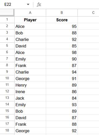
In the sample data, column A contains player names, and some players appear multiple times. In such cases, only their highest score should be considered.

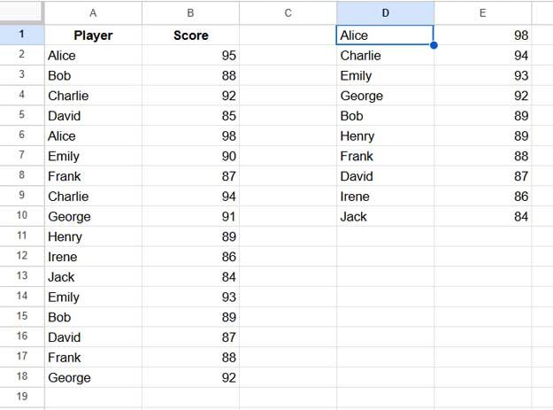
Applying the Formula

To display the top 10 unique players by score, enter one of the formulas above in D1 (if columns D and E are empty). The results will populate in D1:E10.

Example: Find top 10 unique names by score in Google Sheets

How the Formula Works

Below is an explanation of how both formulas work. They are simple to understand—let’s dive in!

SORT + SORTN Method

SORT(A2:B, 2, FALSE): Sorts the scores in descending order (highest to lowest).
SORTN(..., 10, 2, 1, TRUE): Selects top 10 unique names, keeping only their highest score.
SORT(..., 2, FALSE): Ensures the results remain sorted by score.

QUERY Method

group by Col1: Groups rows by player names (removes duplicates).
max(Col2): Extracts each player’s highest score.
order by max(Col2) desc limit 10: Sorts scores in descending order and selects the top 10.

As a side note, between the two functions, I prefer the powerful SORT and SORTN combo over QUERY, as it performs better. QUERY processes structured queries similar to SQL, which can slow performance when working with very large datasets or applying multiple queries to the same dataset.

How to Find the Top 5 Unique Names by Score

If you need the top 5 instead of the top 10:

In SORTN, replace 10 with 5.
In QUERY, replace limit 10 with limit 5.

Example: =SORT(SORTN(SORT(A2:B, 2, FALSE), 5, 2, 1, TRUE), 2, FALSE)

That’s it! You can now easily find the top unique names based on score in Google Sheets.

FAQ: Common Questions About Ranking in Google Sheets

How do I rank without duplicate names in Google Sheets?

Use SORTN or QUERY with MAX(B) to remove duplicates and keep only the highest score.

Can I find the top 10 without using QUERY?

Yes! Use SORTN(SORT(A2:B,2,FALSE),10,2,1,TRUE) to get the top 10 unique names by score.

How do I assign ranks after finding the top 10?

You can use the RANK.EQ or RANK.AVG functions alongside the formulas above. For example, after clearing F1:F, enter the following formula in cell F1.

=ArrayFormula(IFNA(RANK.EQ(E1:E, E1:E)))