TO_PURE_NUMBER Function in Google Sheets

The TO_PURE_NUMBER function in Google Sheets converts formatted numbers into plain numerical values while keeping other values the same.

You can apply various formatting to a number, such as date, time, percentage, scientific, accounting, currency, rounded, etc. The TO_PURE_NUMBER function helps you get the underlying value.

You can use the TO_PURE_NUMBER function for data cleaning when you have imported data in your spreadsheet. It is also useful when exporting data to other software where you want pure numerical values for compatibility. Most importantly, it ensures that all numerical data is in a consistent format to help compare values.

In some functions, such as QUERY, you might find it challenging to remember the correct usage of date and datetime literals. In such cases, you can convert those values to pure numbers and use them as numerical literals.

Note: The TO_PURE_NUMBER function operates exclusively on numerical values and returns the original content for non-numeric data.

TO_PURE_NUMBER Function Syntax

Syntax:

TO_PURE_NUMBER(value)

value – Usually a reference to a cell whose content is to be converted to a pure number. You can hardcode the value to convert as well, but this is less common.

When you specify an array in value, use the ARRAYFORMULA function if the TO_PURE_NUMBER function is not used with SORT, SORTN, FILTER, or INDEX functions. These are some array functions that do not require ARRAYFORMULA for the formula expressions within them.

Examples

The following formula will return 0.25:

=TO_PURE_NUMBER(25%)

If you enter 25% in cell B2, you can use it as:

=TO_PURE_NUMBER(B2)

Let’s convert an array of values in A2:A into pure numbers using the TO_PURE_NUMBER function in cell B2:

=ArrayFormula(TO_PURE_NUMBER(A2:A))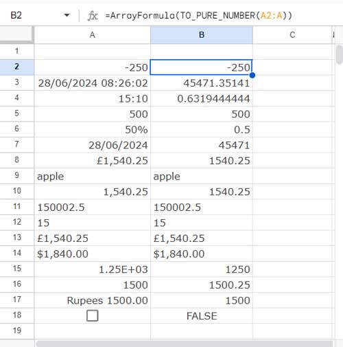

A2:A contains various formatted numbers such as currency, date, time, datetime, custom formatted numbers, text, tickbox, etc. Wherever the ‘value’ is not a number, such as text, the TO_PURE_NUMBER function returns that value without any modification.

How the TO_PURE_NUMBER Function Differs from the N Function

There are three key differences between the TO_PURE_NUMBER and N functions:

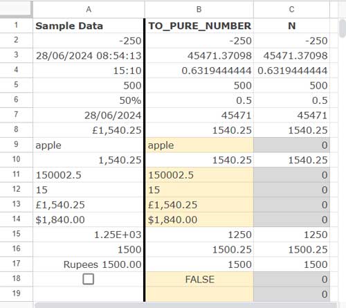
Comparison of TO_PURE_NUMBER and N functions in Google Sheets

Boolean Values:
- N returns 1 for TRUE and 0 for FALSE, whereas TO_PURE_NUMBER returns TRUE or FALSE directly. This is evident when using a tickbox.
- Example: An unticked tickbox in cell A18 will return FALSE with =TO_PURE_NUMBER(A18), but 0 with =N(A18).
Text Values:
- N returns 0 for text values, whereas TO_PURE_NUMBER returns the text itself.
- Example: If cell A9 contains the text “apple”, =TO_PURE_NUMBER(A9) returns “apple”, while =N(A9) returns 0.
Blank Cells:
- N interprets a blank cell as 0, whereas TO_PURE_NUMBER returns an empty cell.
- Example: If cell A19 is blank, =TO_PURE_NUMBER(A19) returns an empty cell, while =N(A19) returns 0.

These differences are crucial in various scenarios. For example, when using MMULT with an open range, you might use N around the arrays to avoid matrix multiplication errors caused by empty cells.

TO_PURE_NUMBER vs Automatic Number Formatting in Google Sheets

If you prefer not to use a formula-oriented approach to obtain pure numbers, you can use Format > Number > Automatic formatting. However, it’s important to understand the differences.

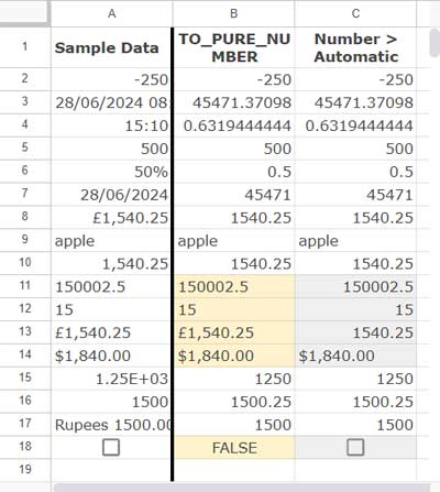
When using this approach, a tickbox will remain as a tickbox, unlike the TO_PURE_NUMBER function where it will be treated as TRUE or FALSE.

Text formatted numbers (except those starting with ') and currencies (set as default in your sheet) will be converted to pure numbers. In contrast, the TO_PURE_NUMBER function will treat them as text.