


")


")

")
")
 in Excel & Google Sheets")


While there’s no built-in SUMUNIQUEIFS function in Google Sheets, we have effective workarounds to sum unique values based on multiple criteria.
While COUNTUNIQUEIFS is designed to count unique values with multiple criteria, a hypothetical SUMUNIQUEIFS function might not be as universally applicable for summing values. This is because, in certain scenarios, users might need to sum all values, including duplicates, rather than just unique ones.
To achieve SUMUNIQUEIFS-like functionality, we’ll explore adaptable formula combinations that address different summing needs.
In this guide, we’ll explore two potent formulas for summing unique values with multiple criteria in Google Sheets:
- Formula 1: Filter, then Unique the table including the sum column.
- Formula 2: Filter, then Unique the table excluding the sum column.
Sample Data
The following sample data is ideal for testing both formula options:
| Item | Category | Quantity | Region |
| Apple | Fruit | 1 | North |
| Apple | Fruit | 5 | North |
| Mango | Fruit | 2 | North |
| Mango | Fruit | 2 | North |
| Avocado | Fruit | 8 | North |
| Avocado | Fruit | 4 | North |
| Orange | Fruit | 3 | South |
| Pear | Fruit | 6 | South |
You may copy-paste this data into cell range A1:D9 in your Google Sheets for testing the SUMUNIQUEIFS workaround solution.
SUMUNIQUEIFS Workaround in Google Sheets: Unique Criteria Columns and Sum Column
This method is useful when you wish to avoid removing duplicate records (rows) from the table temporarily and still perform a conditional sum, excluding those duplicates.
Problem: Calculate the total quantity of all fruits in the north region, excluding duplicate records.
Criteria: B2:B = “Fruit” and D2:D = “North”
Reviewing the sample data above, you’ll notice that only one record is a duplicate, row #5 (a duplicate of row #4).
Formula:
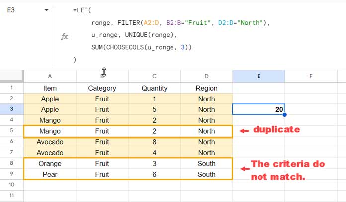
=LET(
     range, FILTER(A2:D, B2:B="Fruit", D2:D="North"),
     u_range, UNIQUE(range),
     SUM(CHOOSECOLS(u_range, 3))
)
Result: This formula will return 20.
Anatomy of the formula:
FILTER(A2:D, B2:B="Fruit", D2:D="North"): FILTER filters the table range A2:D (excluding the header row) based on the specified criteria.LET(range, …): LET names the filter formula with the identifier ‘range.’UNIQUE(range): UNIQUE returns the unique records in the ‘range.’LET(…, …, u_range, …): Names the UNIQUE formula with the identifier ‘u_range.’SUM(CHOOSECOLS(u_range, 3)): The CHOOSECOLS function extracts the third column in ‘u_range’ (the quantity column), and the SUM function totals it.
The above example demonstrates a SUMUNIQUEIFS workaround in Google Sheets, providing a total based on criteria while excluding duplicate rows (records).
SUMUNIQUEIFS Workaround in Google Sheets: Unique Criteria Columns Only
This SUMUNIQUEIFS workaround method in Google Sheets is useful when you want to find the total of the first occurrence of records based on specific criteria.
Problem: Calculate the total quantity of all fruits in the north region, considering unique fruits (not unique records/rows).
Criteria: B2:B = “Fruit” and D2:D = “North”
Formula:
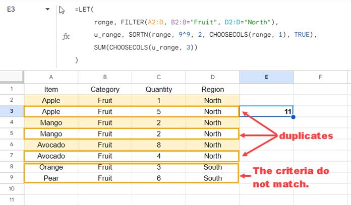
=LET(
     range, FILTER(A2:D, B2:B="Fruit", D2:D="North"),
     u_range, SORTN(range, 9^9, 2, CHOOSECOLS(range, 1), TRUE),
     SUM(CHOOSECOLS(u_range, 3))
)
Result: 11
Anatomy of the formula:
FILTER(A2:D, B2:B="Fruit", D2:D="North"): Filters the table range A2:D (excluding the header row) based on the specified criteria.LET(range, …): Names the filter formula with the identifier ‘range.’SORTN(range, 9^9, 2, CHOOSECOLS(range, 1), TRUE): SORTN returns the unique records in the ‘range’ based on the fruits column.- Where:
rangeis the range to evaluate.9^9is the maximum number of rows in the result.2tie-mode to remove duplicates.CHOOSECOLS(range, 1)is the column to value for duplicates, which is the fruit column. The CHOOSECOLS here returns the first column from the ‘range’.TRUEis the sort order, representing ascending order.
- How do we come to “CHOOSECOLS(range, 1)”?
- We avoid using the criteria columns since they all contain the same data after applying the filter. The remaining columns are the quantity column and the fruit column. Thus, we select the fruit column using the format
CHOOSECOLS(range, 1). - If you have additional columns in your table, aside from the criteria columns and the sum column, you can combine them using the format
CHOOSECOLS(range, 1)&CHOOSECOLS(range, n). Replace ‘n’ with the corresponding column index number. SORTN will then use this column or the combination of columns to remove duplicates.
- We avoid using the criteria columns since they all contain the same data after applying the filter. The remaining columns are the quantity column and the fruit column. Thus, we select the fruit column using the format
- Where:
LET(…, …, u_range, …): Names the UNIQUE formula with the identifier ‘u_range.’SUM(CHOOSECOLS(u_range, 3)): The CHOOSECOLS function extracts the third column in ‘u_range’ (the quantity column), and the SUM function totals it.
The above approach provides an alternative SUMUNIQUEIFS method to sum unique values based on multiple criteria in Google Sheets.
Practical Use of SUMUNIQUEIFS Workaround in Google Sheets
The above two SUMUNIQUEIFS methods in Google Sheets offer effective ways to conditionally sum tables that may contain duplicates. Duplicate records in a table can arise from various reasons, including:
- Data Entry Errors.
- Joining Tables (left, right, inner, or full joins).
- Integrating Data from Various Sources.
- Collaborated Sheets.
- Multiple Submissions of Google Forms Data.
- And many more.
When you find that your table requires cleanup but still wants to perform conditional sum calculations, you can try the above formulas.
The first formula removes duplicate rows before summing from the selected range, while the second formula eliminates duplicates from your preferred non-criteria columns.
Implementing these formulas in your Sheets may require some basic understanding of Google Sheets functions.
Resources: