The combined use of SUMIF with VLOOKUP in Google Sheets might seem intriguing, right? My first priority is to help you understand the relevance of this combination.

We use SUMIF instead of SUM to sum a column based on a specific condition. For example, you can use the SUM function to get the total sales. But when you want to sum the total sales of a particular salesperson, SUMIF is the function you can rely on. Let me quickly explain the difference between SUM and SUMIF.

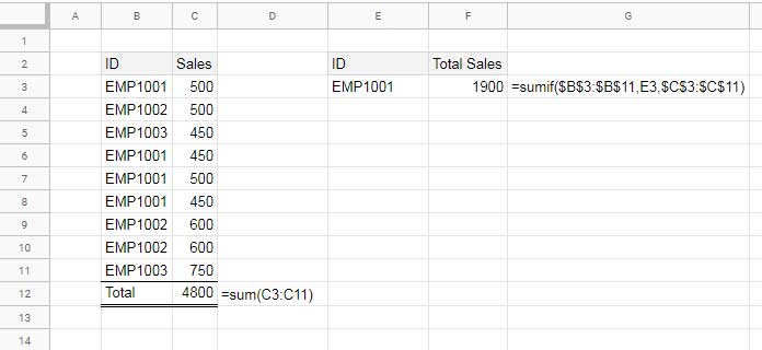
Assume you have employee IDs in column B, ranging from B3:B11, and corresponding sales figures in column C, ranging from C3:C11.

To get the total sales, you can use =SUM(C3:C11). To get the total sales of a particular employee using their ID, e.g., “EMP1001”, you can use the following formula: =SUMIF(B3:B11, "EMP1001", C3:C11).

However, in this case, you might not know the employee ID but only their name. In that situation, you can first use VLOOKUP to look up the employee’s name and return their ID from another table, then use that ID as the criterion in SUMIF. That’s the concept behind combining SUMIF with VLOOKUP, and we’ll explore it below.

Step 1: Assigning ID to Name

Let’s start with the syntax of the SUMIF function:

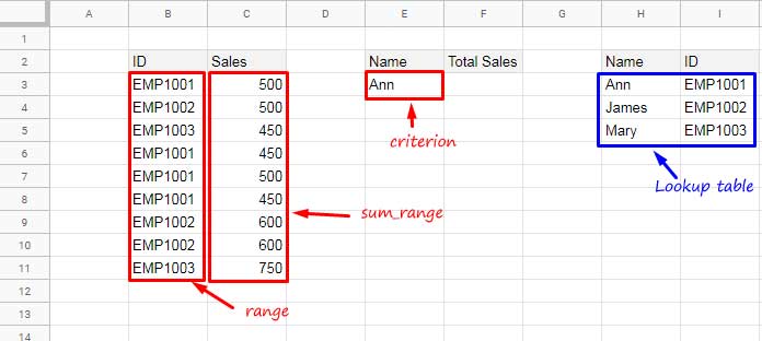
SUMIF(range, criterion, [sum_range])

In our sample data, the range is B3:B11 and the sum_range is C3:C11.

You want to find the sales amount for one of your employees, “Ann.”

If you use =SUMIF(B3:B11, "Ann", C3:C11), the result would be 0 because the criterion “Ann” is not present in the range.

First, we need to find Ann’s ID so that we can use that ID in the SUMIF function.

In a second table, you have names in H3:H5 and corresponding IDs in I3:I5.

How do we assign IDs to names?

You can use the following VLOOKUP formula to look up the name in H3:I5 and return the corresponding ID:

=VLOOKUP(E3, H3:I5, 2, 0)

This formula searches for the name in cell E3 in the first column of H3:I5 and returns the ID from the second column.

The syntax of VLOOKUP is VLOOKUP(search_key, range, index, [is_sorted]).

Step 2: Combining SUMIF with VLOOKUP

The next step is to use the VLOOKUP formula as the criterion in the SUMIF function. Here’s how you can combine SUMIF and VLOOKUP:

=SUMIF(B3:B11, VLOOKUP(E3, H3:I5, 2, 0), C3:C11)

The SUMIF function filters the rows matching the criterion returned by VLOOKUP in the range B3:B11 and returns the sum of the corresponding values in the range C3:C11.

This is the correct way to use SUMIF with VLOOKUP in Google Sheets.

Additional Tip: Using SUMIF with VLOOKUP and Multiple Criteria

How do you find the sales amounts of Ann and James separately or combined?

In the example above, the name “Ann” is in cell E3. You want to keep that name in E3 and enter the next criterion, “James,” in E4.

To achieve this with the SUMIF and VLOOKUP combination, replace E3 within VLOOKUP with E3:E4, and enter the formula as an array formula:

=ArrayFormula(SUMIF(B3:B11, VLOOKUP(E3:E4, H3:I5, 2, 0), C3:C11))

This will return the sales amounts of Ann and James in two cells, vertically. To get the total sales of Ann and James combined, you can wrap this formula with SUM:

=ArrayFormula(SUM(SUMIF(B3:B11, VLOOKUP(E3:E4, H3:I5, 2, 0), C3:C11)))

Resources

• SUMIFS with XLOOKUP in Excel and Google Sheets
• SUMIF IMPORTRANGE in Google Sheets – Examples
• SUMIF with ARRAYFORMULA in Filtered Data in Google Sheets
• Using VLOOKUP to Sum Multiple Rows in Google Sheets