SUMIF with Multiple Criteria in Same Column

Need to conditionally sum a column with SUMIF based on multiple criteria in the same column? Here’s how to do it efficiently in Google Sheets!

When using multiple criteria in the same column, a typical approach is to write separate SUMIF formulas for each criterion and add them together, like this:

=SUMIF(range, criterion1, sum_range) + SUMIF(range, criterion2, sum_range)

While this works, there’s a simpler and more efficient way:

=ArrayFormula(SUMIF(range, {criterion1; criterion2; ...}, sum_range))

Let’s compare both methods to show the benefits of the recommended formula.

Table of Contents

SUMIF with Multiple Criteria (Standard Way)

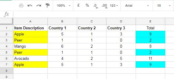
Let’s say you want to find the total quantities for the fruits “Apple” and “Pear” in a sample dataset. The fruit names are in column A, and the quantities are in column E. Using separate SUMIF formulas, the expression would look like this:

=SUMIF(A2:A7, "Apple", E2:E7) + SUMIF(A2:A7, "Pear", E2:E7)

This results in a total of 22.

While this approach works, it has a drawback: you must create a separate SUMIF formula for each criterion.

SUMIF with Multiple Criteria in the Same Column - Method 1

SUMIF with Multiple Criteria (Optimal Method)

Now, let’s combine both criteria into a single SUMIF formula using an array and ArrayFormula:

=ArrayFormula(SUM(SUMIF(A2:A7, {"Apple"; "Pear"}, E2:E7)))

Result: 22

In this formula:

We list the criteria within curly brackets {}.
ArrayFormula processes each criterion in the array.
Wrapping it in SUM combines the totals for each criterion.

If you remove the SUM function, the formula returns separate totals for each item in different cells.

When specifying multiple criteria, you can also use the VSTACK or HSTACK functions instead of array constants:

=ArrayFormula(SUM(SUMIF(A2:A7, VSTACK("Apple", "Pear"), E2:E7)))
=ArrayFormula(SUM(SUMIF(A2:A7, HSTACK("Apple", "Pear"), E2:E7)))

These are the most efficient ways to use SUMIF with multiple criteria in the same column in Google Sheets.

Bonus Tip: Group-Wise Summary with SUMIF in Google Sheets

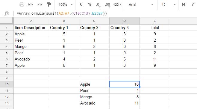
You can extend this array-based SUMIF formula to generate a summary by category. Here’s how:

Use the UNIQUE function to extract unique items (e.g., unique fruit names) in a column:

=UNIQUE(A2:A7)

Then, apply an ArrayFormula-enhanced SUMIF to total each unique item:

SUMIF with Multiple Criteria in the Same Column and Individual Results

=ArrayFormula(SUMIF(A2:A7, C10:C13, E2:E7))

Advanced Users: You can combine UNIQUE and SUMIF in a single formula to generate both the unique items and their totals together:

={UNIQUE(A2:A7), ArrayFormula(SUMIF(A2:A7, UNIQUE(A2:A7), E2:E7))}

This formula will display the unique items in one column and their respective totals in the adjacent column.

Final Thoughts

Try these formulas in your sheet to understand how they work and optimize your calculations. With these techniques, you can efficiently sum based on multiple criteria in the same column and even generate grouped summaries.

Hope this helps you master SUMIF with multiple criteria in Google Sheets!