


")


")

")
")
 in Excel & Google Sheets")


When you use the SUMIF function in merged cells in Google Sheets, it may return an incorrect sum if the cells in the range are merged while the sum range is not.
To correctly use SUMIF with merged cells, you can apply the following formula:
=SUMIF(ARRAYFORMULA(LOOKUP(ROW(range), IF(LEN(range), ROW(range)), range)), criterion, sum_range)Formula Components
- range – The range to filter based on the criterion.
- criterion – The condition to filter the range.
- sum_range – The range to sum based on the criterion.
Understanding Merged Cells in Google Sheets
Unlike database applications, Google Sheets allows merging cells, which you can find under the Format menu. However, merging cells can disrupt the structured nature of a dataset, making it difficult to use functions like SUMIF, FILTER, QUERY, and others.
If your dataset contains merged cells, standard SUMIF formulas may return incorrect results. Below is an example illustrating this issue and the correct workaround.
Example: SUMIF Returning Incorrect Results
Consider the following dataset:
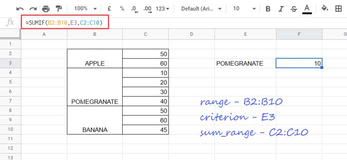
If you use a regular SUMIF formula like:
=SUMIF(B2:B10, E3, C2:C10)It may return 10 instead of 100 (10+20+30+40) for the criterion “POMEGRANATE” in cell E3.
If you unmerge the cells and structure the data as a proper table, the formula works correctly.
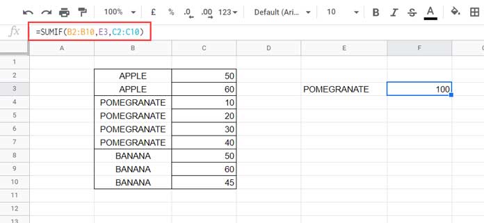
However, if you want to keep merged cells, you need to modify the formula.
Correct SUMIF Formula for Merged Cells
Replace the above formula with:
=SUMIF(ARRAYFORMULA(LOOKUP(ROW(B2:B10), IF(LEN(B2:B10), ROW(B2:B10)), B2:B10)), E3, C2:C10)This version ensures that merged cells are properly accounted for.
Formula Explanation
Since the range contains merged cells, we create a virtual range using:
ARRAYFORMULA(LOOKUP(ROW(B2:B10), IF(LEN(B2:B10), ROW(B2:B10)), B2:B10))This formula fills empty merged cells with values from the preceding non-empty cell. The adjusted data looks like this:
Apple
Apple
Pomegranate
Pomegranate
Pomegranate
Pomegranate
Banana
Banana
Banana
The SUMIF function then correctly sums values based on the adjusted range.
Conclusion
Using this approach, you can correctly apply SUMIF to merged cells in Google Sheets without restructuring your dataset. This method ensures accurate results even when cells are merged.
Related Resources
- Copy-Paste Merged Cells Without Blank Rows/Spaces in Google Sheets
- Uncover Merged Cell Addresses in Google Sheets
- How to Use COUNTIF or COUNTIFS in Merged Cells in Google Sheets
- How to Use VLOOKUP in Merged Cells in Google Sheets
- Filtering When Columns Contain Merged Cells in Google Sheets
- XLOOKUP in Merged Cells in Google Sheets
The formula is terrific as I continue to inevitability deal with the team merging cells in the Google Sheets we share.
I’m having trouble with one thing and am not sure how to revise the formula to address it.
I have 24 columns, and I want a total of column I, which has dollar amounts based on the date in column T.
=SUMIF(ArrayFormula(lookup(row(T2:T4416),if(len(T2:T4416),row(T2:T4416)),T2:T4416)),B2,I2:I4416)
Cell B2 = 7/18/2022
Columns
Row # | Column I | Column T
3089 | $2,000 | 7/18/2022
3094 | $2,222 | (blank cell)
If I enter a “-” in the blank cell, it calculates the formula to only $2,000, which is the total I’m after.
Any suggestion on how to fix this is greatly appreciated!
Many thanks!
Hi, LeSha T.,
I assume you have merged cells in T2:T4416. Otherwise, you might have used a simple formula like this.
=sumif(T2:T4416,B2,I2:I4416)Now, to solve the issue, you must understand the reason.
In a vertically merged range, only the first cell contains the value. All other cells are blank.
My formula fills the blank cells in cell range T2:T4416 with the dates from just above cells.
While doing so, the formula fills all blank cells, whether within merged range or standalone.
So as you have suggested, leaving a hyphen in the cell that you want to skip will solve the issue.
But it’s not practical with several such cells. So do as follows.
1. Select T2:T4416.
2. Go to Format > Number > Plain Text (later, we will revert to date).
3. Go to Edit > Find and Replace.
4. In the “Find” field, input
^([\t]*)$and put a hyphen character in the “Replace with” field.5. Check “Match case” and “Search using regular expressions” and Done.
6. Then revert T2:T4416 to date.