


")


")

")
")
 in Excel & Google Sheets")


Most of the time, when we use SUMIF in Google Sheets, we think vertically — criteria in one column, numbers in another. But what if your data runs across rows instead of down columns?
For example, think about sales data by quarter. The quarters are in the header row, and the sales figures for each product sit across the row. That’s when you need to use SUMIF horizontally in Google Sheets.
In this guide, I’ll show you how to:
- Sum values across columns based on one criteria.
- Apply multiple criteria (like Q1 + Q2).
- Spill results across multiple rows without dragging formulas.
- Handle open ranges without clutter.
Sample Data
Here’s the dataset we’ll use. It shows sales for four products across Q1 to Q4 in both 2023 and 2024.
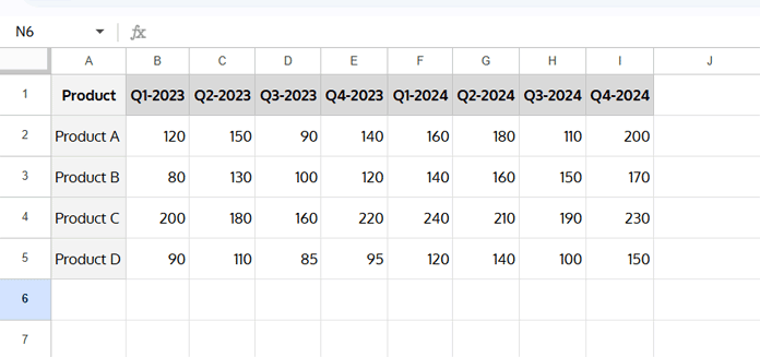
Here, the header row (Q1–Q4 for each year) will be our criteria range, and each product row will be our sum range.
Example 1: SUMIF Horizontally with a Single Criterion
Let’s start simple: total sales for Product A in Q1 across 2023 and 2024.
=SUMIF($B$1:$I$1, "Q1*", B2:I2)What’s happening here?
$B$1:$I$1→ header row (criteria range)."Q1*"→ criteria (matches Q1 in both years).B2:I2→ sales data for Product A.
Result: 120 + 160 = 280
Now, how do we extend this to all products? Two options:
Option 1 — Drag down
Copy the formula down to apply it to Products B, C, and D.
Option 2 — Use BYROW for a spill
=BYROW(B2:I5, LAMBDA(r, SUMIF(B1:I1, "Q1*", r)))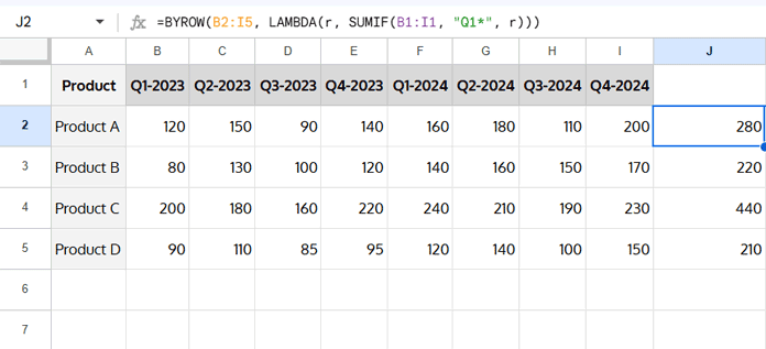
This way, you don’t have to copy formulas — the results spill automatically.
For open ranges with trailing blanks, use this version to skip unwanted zeros:
=BYROW(B2:I, LAMBDA(r, LET(total, SUMIF(B1:I1, "Q1*", r), IF(total=0,,total))))Example 2: SUMIF Horizontally with Multiple Criteria
Now let’s say we want to total Q1 and Q2 together.
=SUMPRODUCT(SUMIF($B$1:$I$1, HSTACK("Q1*", "Q2*"), B2:I2))
Here’s the trick:
- HSTACK → creates multiple criteria (Q1 and Q2).
SUMIF→ returns separate sums for each.- SUMPRODUCT → adds them together in one step.
This works for one row (e.g., Product A).
Want to get results for all products? Here are two approaches:
Option 1 — Drag down
Just drag the formula down to cover Product B, C, and D.
Option 2 — Use BYROW for a spill
=BYROW(B2:I5, LAMBDA(r, SUMPRODUCT(SUMIF(B1:I1, HSTACK("Q1*", "Q2*"), r))))This way, all product totals spill automatically without copying formulas.
If your range extends beyond data and may include empty cells, try this version:
=BYROW(B2:I, LAMBDA(r, LET(total, SUMPRODUCT(SUMIF(B1:I1, HSTACK("Q1*", "Q2*"), r)), IF(total=0,,total))))Example 3: Yearly Totals
Sometimes, you don’t want just quarters — you want a whole year.
For 2023 totals (per product):
=SUMIF(B1:I1, "*2023", B2:I2)For 2024 totals:
=SUMIF(B1:I1, "*2024", B2:I2)Super clean!
Wrapping Up
Using SUMIF horizontally in Google Sheets unlocks a lot of flexibility when your data is structured across rows instead of columns.
Here’s what you learned today:
- How to apply a single criterion (like Q1).
- How to sum with multiple criteria (like Q1 + Q2).
- How to use
BYROWto spill results across multiple rows. - How to grab totals for an entire year.
Next time you’re tracking sales, budgets, or KPIs that run across a timeline, you’ll know exactly how to handle it.
Sample Google Sheet
Related Reading
- How to Use Dynamic Ranges in SUMIF Formula in Google Sheets
- SUMIF with Multiple Criteria in Same Column – Google Sheets
- Multiple Sum Columns in SUMIF in Google Sheets
- Multiple Criteria SUMIF Formula in Google Sheets (Beyond Basic SUMIF)
- Sum of Matrix Rows or Columns Using SUMIF in Google Sheets
- How to Calculate a Horizontal Running Total in Google Sheets