 in Google Sheets")

")

")


")


")


Using my workaround, you can sort pivot table rows, not by the first column, but by the nth column in Google Sheets.
That means, presently, there is no such built-in option available within Sheets’ pivot table editor. So we require to follow the workaround.
Assume our pivot table report, not the source data, has the following table structure, i.e., “Item,” “Supplier,” “P.O. Date,” and “SUM of Order Qty.”
So, there are three ‘Rows’ fields (first three) and one ‘Values’ field (last one).
I want to sort the pivot table rows by “P.O. Date.” Since it’s the third column, we won’t get the required output.
Why?
It’s because the sorting will be in the following order, i.e., Item/SUM of Order Qty -> Supplier/SUM of Order Qty -> P.O. Date/SUM of Order Qty.
The “SUM of Order Qty” is a ‘Values’ (calculation) field. So you will get this option against each column for sorting.
Here is an example of sorting pivot table rows, not by the first column, but by the nth column in Google Sheets.
Sample Data
I have the following mockup purchase order details in cell range A1:F8.
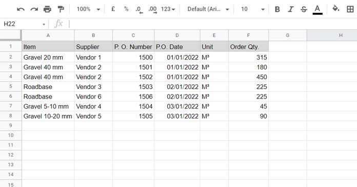
Note:- You can copy this data from my sample sheet below.
I want to group this purchase order by Items -> Supplier -> P.O. Date and get the sum of “Order Qty.”
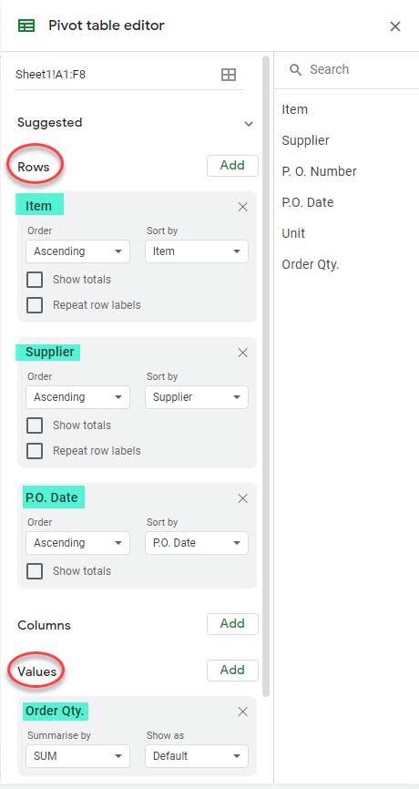
For that, we can follow the below pivot table settings.
- Drag and drop the above first three fields under “Rows.”
- Then drag and drop the last field, i.e., the Order Qty. under “Values.”
Please refer to the below pivot table editor screenshot with the said settings.
It will insert the below pivot table report in your Sheet.
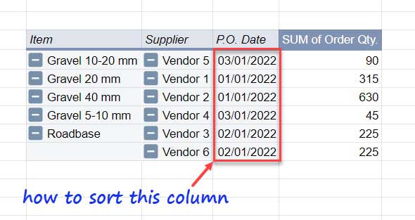
Note:- Please see cell J15 in my sample sheet above.
As you can see, the P.O. Dates are not in any order. It’s because the other two fields supersede its sorting.
I want the “P.O. Date” column sorted in ascending or descending order.
To get that, you should know how to sort pivot table rows by nth column in Google Sheets.
Workaround to Sort Pivot Table Rows, Not by the First Column in Google Sheets
The workaround requires a helper column.
The sample mockup data has six columns from column A to F.
We require one more column. We will use column G for that which is currently empty.
To sort pivot table rows, not by the first column, but by the nth column in ascending order, we can use an array formula in G1.
But the formula depends on the formatting of column D (P.O. Date).
Sorting Pivot Table Rows by Nth Date/Number/Time Column
We can use a RANK-based formula if the nth column is a date, number, or time column.
In our case, we have a date column. So we can use the below RANK formula in cell G1. It’s for sorting the nth column in ascending order.
=ArrayFormula(ifna({"Helper";rank(D2:D,D2:D,1)}))To sort the pivot table by the nth column in descending order, use the below formula instead.
=ArrayFormula(ifna({"Helper";rank(D2:D,D2:D,0)}))Now open the pivot table editor and drag and drop the new field “Helper” above the “Item.”
That’s the only change required there.
Finally, within the pivot table report, you may hide the first column, i.e., “Helper.”
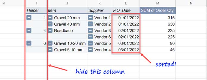
Note:- Please check cell I1 on my mockup sample sheet.
Sorting Pivot Table Rows by Nth Text Column
Sometimes the nth column may be a text column. So the RANK formula may return #VALUE!.
In that scenario, use the below COUNTIF array formula.
Assume column D contains texts, not dates. Then use either of the below formulas in cell G1.
Ascending:
=ArrayFormula({"Helper";if(D2:D="",,COUNTIF(D2:D,"<="&D2:D))})Descending:
=ArrayFormula({"Helper";if(D2:D="",,COUNTIF(D2:D,">="&D2:D))})This way, we can sort pivot table rows, not by the first column, but by the nth column in Google Sheets.
Resources
- How to Sort Pivot Table Grand Total Columns in Google Sheets.
- How to Sort Pivot Table Columns in the Custom Order in Google Sheets.
- Filter Top 3 Values in Each Group in Pivot Table – Google Sheets.
- Rolling 7, 30, 60 Days in Pivot Table in Google Sheets.
- How to Filter Top 10 Items in Google Sheets Pivot Table.
- Filter Multiple Values in Pivot Table in Google Sheets.
- All About Calculated Field in Pivot Table in Google Sheets.
In case the PO dates of the same item of different vendors are different, doing so the Item can not be grouped anymore, right?
Hi, Jimmy,
In that case, place the field Helper between Item and Supplier, and hide it.