How to Properly Sort Alphanumeric Values in Google Sheets

Published on

There are two different kinds of formulas/methods for alphanumeric sort. With or without using a helper column we can sort alphanumeric values in a column in Google Sheets.

The first method supports point # 1 below. The second method supports all three points.

  1. Numbers prefixed left to the text in alphanumeric values.
    • Example: 32109AB
  2. Letters prefixed left to numbers in alphanumeric values.
    • Example: ZZ32110
  3. Mixed types of alphanumeric values, a mix of the above two, in a column.

Let’s start with the method one.

Sort Alphanumeric Data Using Helper Column in Google Sheets (Numbers Prefixed Left)

If numbers are prefixed in all the alphanumeric values, then we can very easily sort such an alphanumeric value column in Google Sheets.

For this, I have a helper column-based formula that many of you can easily follow. But I won’t call it a ‘proper’ formula to sort alphanumeric data. Why?

I’ll explain that under the pros and cons section below.

Assume the column A, for example, the array A1:A10, contains alphanumeric values with numbers prefixed left.

In this case, just sort this data in any column (I am using column H) using the below SORT formula.

The Formula in Cell H1 in Helper Column H:

=sort(A1:A)

Convert these sorted values to pure text using the To_text function in column F (cell F1).

Here is the To_text formula.

=ArrayFormula(to_text(H1:H10))

This converts the sorted alphanumerics to pure text. Wrap the just above formula with Sort (feel free to remove the ArrayFormula function at it is not compulsory to use within Sort).

=sort(to_text(H1:H10))

This way we can easily sort the number prefixed alphanumeric values in Google Sheets.

If you can’t understand my explanation properly, here is the illustration.

Sort Number Prefixed Alphanumeric Values in Google Sheets

Here are the pros and cons of using the above formula to sort alphanumeric values in a column in Google Sheets.

Pros and Cons of the Formula

Pros:

  • Simple to understand and use.

Cons:

  • The formula requires a helper column to work.
  • It only supports alphanumeric data which has formatted as numbers prefixed.
  • The other issue is the number of digits.
    • The numbers should follow the same pattern, I mean the same number of digits in all the values. For example, use 099 instead of 99 if the majority of the values have 3 digit numbers.

Can you suggest a formula that properly sorts alphanumeric values in Google Sheets? I mean a formula that without the above cons.

Yes! We can use a Regex based Sort formula for this. I’ll explain it step by step below.

Proper Formula to Sort Alphanumeric Values in Google Sheets (No Issue with Prefix/Suffix)

Let us start with the logic.

You may find the logic little complex to understand. But the formula is simple and you can understand the logic clearly later from the formula part. Just read on.

Logic:

Using Regexextract, a popular text function in Sheets, first I will extract the numbers only from each row (from the alphanumeric column A).

Then we can sort the column A using the extracted numbers as the sort_column.

Syntax:

SORT(range, sort_column, is_ascending)

As you may know, the Sort function in Google Sheets supports column index or a range outside the ‘range’ as the sort column.

The above two actions should be performed on a sorted alphanumeric column A. Why?

For our example, I am taking a dataset that contains ‘mixed’ type of alphanumeric characters.

Sample Data:

Sample Data - Alphanumeric Sort

Before suing Regex you might sort this range (A1:A10) using the Data menu Sort range by column A, A-Z.

This will help you to sort the alphanumeric values like “PQ32115” above “VW32115” in the final formula output.

In my example, I am not sorting the data manually as above mentioned. Instead, I am using the SORT function within my formula.

In the first step, I will extract numbers from the alphanumerics in column A.

Extract Numbers from Alphanumeric Data in Sheets

Using the below formula in cell D1 we can extract all the numbers from column A.

=ArrayFormula(IFNA(REGEXEXTRACT(sort(A1:A)&"","[0-9]+")*1))

See, I have used sort(A1:A) instead of A1:A in REGEXEXTRACT(sort(A1:A)&"","[0-9]+").

The IFNA is to return blank instead of #N/A error in blank cells and *1 is to convert the extracted numbers which are obviously in text format (Regexextract is a text function) to numbers.

Sort and Extract Numbers from Alphanumeric Data

Here is the second step.

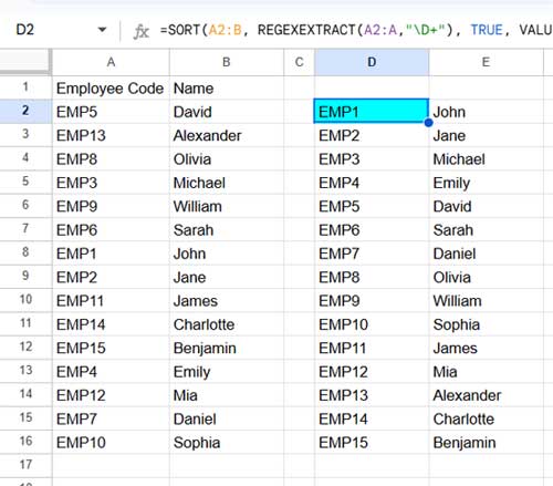
Sort Alphanumeric Values with Extracted Numbers in Google Sheets

If you compare the extracted numbers with the corresponding numbers in the alphanumerics in column A, you won’t find any match! Because I have extracted the numbers after sorting.

Just key =sort(A1:A) in cell C1 and compare the numbers in this column with the numbers in column D. You can see it matches.

Compare Extracted Numbers with Corresponding Column

Here is the final step (you can delete the C1 formula). I am modifying the cell D1 formula as below.

What I am going to do/perform is sorting sorted A1:A sort(A1:A) with the extracted numbers.

=sort(sort(A1:A),IFNA(REGEXEXTRACT(sort(A1:A)&"","[0-9]+")*1),1)
The Perfect Formula to Sort Alphanumeric Values in Google Sheets

The above is the perfect formula to sort alphanumeric values in Google Sheets.

Prashanth KV
Prashanth KV
Your Trusted Google Sheets and Excel Guide Prashanth KV brings a wealth of experience in Google Sheets and Excel, cultivated through years of work with multinational corporations in Mumbai and Dubai. As a recognized Google Product Expert in Docs Editors, Prashanth shares his expertise through insightful blogging since 2012. Explore his blog for practical tips and guidance on maximizing your spreadsheet skills.

How to Extract Numbers from Text in Excel with Regex

You can use the REGEXEXTRACT or REGEXREPLACE functions to easily extract numbers from text...

Using OFFSET and MATCH Together in Google Sheets: Advanced Tips

One powerful and flexible way to look up values is by combining the OFFSET...

How to Use OFFSET and XMATCH Functions Together in Excel

We often use the OFFSET and XMATCH functions together to match a value in...

How to Calculate Maximum Drawdown in Excel and Google Sheets

You can use the following dynamic array formula to calculate maximum drawdown (MDD) in...

More like this

Using OFFSET and MATCH Together in Google Sheets: Advanced Tips

One powerful and flexible way to look up values is by combining the OFFSET...

Running Count with Structured References in Google Sheets

Running a count with structured references is achievable in Google Sheets tables using the...

Running Total with Structured Table References in Google Sheets

You can use two types of formulas to create a running total with structured...

LEAVE A REPLY

Please enter your comment!
Please enter your name here

This site uses Akismet to reduce spam. Learn how your comment data is processed.