Want to simplify conditions in multiple columns in Google Sheets QUERY? Manually writing multiple conditions can be repetitive and error-prone — here’s a smarter way to do it.
Let’s say you want to return only the rows where columns B, C, and D all have values greater than or equal to 90. The basic approach would be:
=QUERY(A1:D, "select * where B >= 90 and C >= 90 and D >= 90", 1)
That works for a few columns. But what if you’re working with 10 or more? Typing each condition manually becomes cumbersome and prone to errors.
🔗 Sample Sheet
To follow along or test the formulas, you can copy this sample Google Sheet.
This tutorial is part of the WHERE Clause in Google Sheets QUERY: Logical Conditions Explained hub, which covers all logical operators, comparisons, and condition-building patterns used in QUERY statements.
A Smarter Way to Simplify AND Conditions in Multiple Columns
To simplify conditions in multiple columns in Google Sheets QUERY, you can build the WHERE clause dynamically using a combination of TEXTJOIN, ARRAYFORMULA, and SEQUENCE.
=QUERY(A1:D, "select * where " & TEXTJOIN(" and ", TRUE, ARRAYFORMULA("Col" & SEQUENCE(3, 1, 2) & ">=90")), 1)How It Works:
SEQUENCE(3, 1, 2)→ generates{2; 3; 4}for columns B, C, D (since column B = Col2). This follows the syntaxSEQUENCE(rows, [columns], [start], [step]), where 3 rows are generated starting from 2."Col" & SEQUENCE(...) & ">=90"→ creates individual conditions.TEXTJOIN(" and ", TRUE, …)→ combines them into one string:"Col2>=90 and Col3>=90 and Col4>=90"
This formula dynamically builds the condition without needing to write each manually — making your formula scalable and easier to maintain.
Why Simplifying Multiple Column Conditions in QUERY Is Useful
- Cleaner formulas for wide datasets
- Easy to audit or change conditions
- Ideal for patterned conditions (e.g., all
>=90,IS NOT NULL, etc.) - Works well with large numbers of columns
Customize It Further
Between Two Values
Want to check if values fall between 90 and 95?
=QUERY(A1:D, "select * where " & ARRAYFORMULA(TEXTJOIN(" and ", TRUE, "Col"&SEQUENCE(3, 1, 2)&">=90 AND Col"&SEQUENCE(3, 1, 2)&"<=95")), 1)Use Different Operators
Simply swap >=90 with any other condition like =100, <85, etc.
Non-Contiguous Columns? No Problem!
You can specify column positions manually using an array instead of SEQUENCE.
=QUERY(A1:G, "select * where " & TEXTJOIN(" and ", TRUE, ARRAYFORMULA("Col" & {2, 4, 6} & ">=90")), 1)Replace AND with OR
Want any of the conditions to be true instead of all?
Just replace " and " with " or " inside the TEXTJOIN function.
Example: Simplify IS NOT NULL Conditions in Multiple Columns in QUERY
Here’s a traditional approach:
=QUERY(A1:D, "select * where B is not null and C is not null and D is not null", 1)Here’s the simplified version:
=QUERY(A1:D, "select * where " & TEXTJOIN(" and ", TRUE, ARRAYFORMULA("Col"&SEQUENCE(3, 1, 2)&" IS NOT NULL")), 1)Again, no need to type out each column manually.
Real-World Use Case: Simplifying Attendance Filters in Google Sheets QUERY
Let’s say you track employee attendance in range A1:AF, where:
- Column A: Employee names
- Columns B to AF: Daily attendance for 31 days (values: P = Present, H = Holiday, A = Absent)
You want to filter employees who were present the entire month (i.e., all days are either P or H — not A).
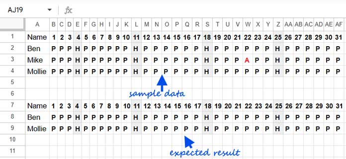
=QUERY(A1:AF, "SELECT * WHERE " & TEXTJOIN(" and ", TRUE, ARRAYFORMULA("(Col"&SEQUENCE(27, 1, 2)&"='P' OR Col"&SEQUENCE(27, 1, 2)&"='H')")), 1)This returns only those rows where none of the attendance values are “A”.
Summary Reference: QUERY Conditions for Multiple Columns
| Condition Type | Formula Snippet |
|---|---|
AND condition | TEXTJOIN(" and ", TRUE, ARRAYFORMULA("Col" & SEQUENCE(...) & ">=90")) |
BETWEEN range | ARRAYFORMULA(TEXTJOIN(" and ", TRUE, "Col"&SEQUENCE(...)&">=90 AND Col"&SEQUENCE(...)&"<=95")) |
IS NOT NULL check | TEXTJOIN(" and ", TRUE, ARRAYFORMULA("Col"&SEQUENCE(...)&" IS NOT NULL")) |
AND + OR mixed logic | TEXTJOIN(" and ", TRUE, ARRAYFORMULA("(Col"&SEQUENCE(...)&"='P' OR Col"&SEQUENCE(...)&"='H')")) |
Conclusion
Manually writing multiple column conditions in Google Sheets QUERY can be a chore — especially with large datasets. But with clever use of TEXTJOIN, ARRAYFORMULA, and SEQUENCE, you can simplify conditions in multiple columns in Google Sheets QUERY and make your formulas cleaner, scalable, and much easier to work with.


No example about how to select more than 1 column.
Hello,
Please see the examples below:
Select A – to select column A
Select * – to select all the columns.
Select A, B – to select the columns A and B
Alternatives (if Query data is an expression)
Select Col1 – to select column 1
Select * – to select all the columns.
Select Col1, Col2 – to select columns 1 and 2.