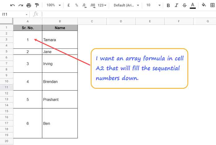
To autofill sequence numbering in merged cells in a column, we can use an array formula in Google Sheets.

For example, I have names in B2:B, and some rows are merged based on the formatting.

Accordingly, I have merged cells in A2:A to match the rows in B2:B.

Now, how do we autofill serial numbers in the merged cells in column A corresponding to the names in column B?

Let’s find out.

Array Formula for Sequence Numbering in Merged Cells

The best solution is to use an array formula in cell A2 to achieve sequence numbering in merged cells A2:A in Google Sheets. I’ll come to that shortly.

Some users follow a non-array method, which is a bit tedious:

• Select A2:A and unmerge the rows (Format > Merge cells > Unmerge).
• In cell A2, enter:
  =IF(LEN(B2), COUNTA($B$2:B2), )
• Drag the formula down until the last row you need (say, up to row #19).
• Then, select B2:B19.
• Right-click and select Copy.
• Right-click on cell A2 and select Paste special > Format only.

It’s a time-consuming process.

Instead, you can use my array formula to auto-fill sequence numbers in a merged column — no need to unmerge A2:A.

Just insert the formula in cell A2, and it will automatically populate the serial numbering in the merged column based on the names in column B.

I have two formula options for you.

1. VLOOKUP to Auto Fill Sequence Numbers in Merged Cells

Array Formula #1:

=ArrayFormula(IFNA(VLOOKUP(ROW(B2:B), {FILTER(ROW(B2:B), LEN(B2:B)), SEQUENCE(COUNTA(B2:B), 1)}, 2, 0)))

Insert the above array formula in cell A2.

It will automatically fill the sequence numbers in a merged column corresponding to the values in B2:B.

Formula Explanation

To understand the VLOOKUP formula, start from the middle — the FILTER part:

FILTER(ROW(B2:B), LEN(B2:B))

This returns the row numbers where there are actual values in B2:B.

Here, LEN(B2:B) checks whether the cell is non-blank.

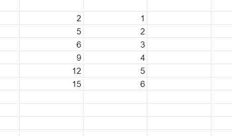
The output will be something like row numbers 2, 5, 6, 9, 12, and 15.

Next, the SEQUENCE part:

SEQUENCE(COUNTA(B2:B), 1)

COUNTA(B2:B) counts the non-blank cells (names) in B2:B. Suppose there are six names — the sequence would generate numbers 1 to 6.

Then, using curly brackets {}, I create a two-column array:

{FILTER(ROW(B2:B), LEN(B2:B)), SEQUENCE(COUNTA(B2:B), 1)}

The result is a two-column table — first with the row numbers and second with the sequence numbers.

Now, VLOOKUP searches the first column (row numbers) for ROW(B2:B) from row 2 downwards.

If it finds a match, it returns the serial number from the second column.

If no match is found, IFNA ensures it leaves the cell blank.

2. Running Count to Auto Fill Sequence Numbers in Merged Cells

Array Formula #2:

=ARRAYFORMULA(IF(LEN(B2:B), COUNTIFS(ROW(B2:B), "<="&ROW(B2:B), LEN(B2:B), ">0" ), ))

Again, just insert this formula into A2.

It will automatically generate serial numbering in merged column A2:A without the need to unmerge anything.

Formula Explanation

This formula uses COUNTIFS and follows a simple running count logic:

• For each row, it checks if the row number is less than or equal to the current row number.
• It also checks if there is a value in column B.

If both conditions are met, it counts how many such rows there are — giving you the sequence numbering in merged cells.

Conclusion

To achieve sequence numbering in merged cells in Google Sheets, you can try either of the above formulas.

Both work great, but depending on how many merged rows you have, one might be faster than the other.

Just insert the formula and forget about manual dragging or formatting!

Resources

• Group Wise Serial Numbering in Google Sheets
• Group-Wise Dependent Serial Numbering in Google Sheets
• Copy-Paste Merged Cells Without Blank Rows/Spaces in Google Sheets
• How to Find the Cell Addresses of the Merged Cells in Google Sheets
• How to Use SUMIF in Merged Cells in Google Sheets
• Sort Vertically Merged Cells in Google Sheets (Workaround)
• Merge and Unmerge Cells and Preserve Values in Google Sheets
• How to Fill Merged Cells Down or to the Right in Google Sheets