The SEQUENCE function is a versatile tool in Google Sheets that allows you to generate sequential numbers in rows, columns, or even as a matrix. Before this function, we often relied on ROW or COLUMN functions, which had certain limitations.
These earlier functions return row or column numbers, but they require a physical range, such as A:A or 1:1.
For example, =ARRAYFORMULA(ROW(A1:A)) in cell B1 will return row numbers from 1 to the last row in the sheet. However, using expressions like {A2:A} with these functions results in a “argument must be a range” error. This makes them less practical in complex formulas where sequence numbers are needed.
This is where the SEQUENCE function in Google Sheets becomes invaluable. Below, you’ll find everything from basic to advanced uses of this function.
Syntax of the SEQUENCE Function in Google Sheets
The syntax for the SEQUENCE function is as follows:
SEQUENCE(rows, columns, start, step)- rows: The number of rows in the resulting sequence.
- columns: (Optional) The number of columns. Defaults to 1.
- start: (Optional) The starting value of the sequence. Defaults to 1.
- step: (Optional) The incremental value. Defaults to 1 and can be a decimal or negative.
Basic Examples of SEQUENCE
1. Single Column Sequence:
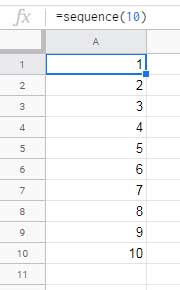
=SEQUENCE(10)This returns the numbers 1 to 10 in a single column.

2. Single Row Sequence:
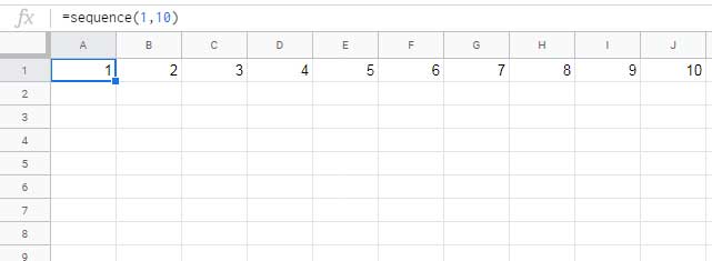
=SEQUENCE(1, 10)This generates the numbers 1 to 10 across a single row.

3. Matrix Sequence:
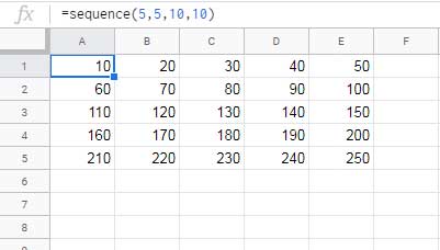
=SEQUENCE(5, 5, 10, 10)This creates a 5×5 matrix, starting at 10 and increasing by 10. The result will look like:

4. Decimal Steps:
=SEQUENCE(10, 1, 1, 0.25)This generates a sequence like: 1, 1.25, 1.5, 1.75, 2, …
5. Negative Sequence:
=SEQUENCE(10, 1, -1, -1)This produces a sequence from -1 to -10.
SEQUENCE with Dates and Times
The SEQUENCE function in Google Sheets works well with date and time functions to generate dynamic sequences. Here are some examples:
1. Date Sequence:
=ARRAYFORMULA(TO_DATE(SEQUENCE(10, 1, "2025/01/01")))This formula generates dates from January 1, 2025, to January 10, 2025. Use DATE(2025, 1, 1) instead of "2025/01/01" for better flexibility.
2. Time Sequence:
=ARRAYFORMULA(SEQUENCE(24, 1, "01:00:00", 1/24))Format the result as Time (Format > Number > Time) to display hours from 01:00:00 to 24:00:00.
3. Month-End Dates:
=ARRAYFORMULA(EOMONTH("2025/01/01", SEQUENCE(12, 1, 0)))This generates the last date of each month in 2025.
4. Month-Start Dates:
=ARRAYFORMULA(EDATE("2024/12/01", SEQUENCE(12))) This outputs the first day of each month in 2025.
Creative Uses of SEQUENCE
1. Alphabet Sequences:
- Lowercase letters
a-z:
=ARRAYFORMULA(CHAR(SEQUENCE(26, 1, CODE("a"))))- Uppercase letters
A-Z:
=ARRAYFORMULA(CHAR(SEQUENCE(26, 1, CODE("A"))))2. Repeat Symbols:
=ARRAYFORMULA(CHAR(SEQUENCE(10, 1, CODE("♥"), 0)))This repeats the heart symbol 10 times in a column.
3. Grouped Numbering:
=ARRAYFORMULA(ROUNDDOWN(SEQUENCE(16, 1, 1, 1/4)))This produces a grouped sequence like: 1, 1, 1, 1, 2, 2, 2, 2, …
4. Dynamic Length Sequence Using MATCH:
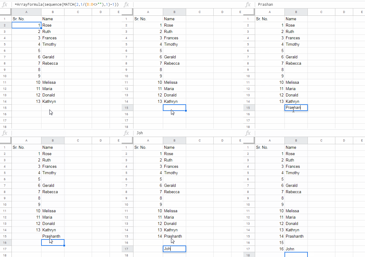
=ARRAYFORMULA(SEQUENCE(MATCH(2, 1/(B2:B<>""), 1))) This formula stops numbering at the last non-blank cell in column B.

Additional Resources
- Backward Sequence Numbering in Google Sheets
- Fill a Column with Sequence of Decimals in Google Sheets
- Generate a Sequence of Months in Google Sheets
- Create Custom Time Slot Sequences in Google Sheets
- Add N Blank Rows to SEQUENCE Results in Google Sheets
- Create a Dynamic Fibonacci Sequence in Google Sheets
- Group-Wise Serial Numbering in Google Sheets
- Group-Wise Dependent Serial Numbering in Google Sheets


Hi,
How do I organize the filing of documents in Google Sheets using serial numbers?
For instance:
From [Control # 001-23] to [Control # 1000-23], how can I manage this in Google Sheets?
In a blank column, enter this formula in the topmost cell:
=ArrayFormula("Control # "&TEXT(SEQUENCE(1000), "000")&"-"&23)I hope that helps.
Hi there!
I would like to know how can I get Dynamic Sequential Numbering in Google Sheets.
=ArrayFormula(sequence(MATCH(2,1/(not(B:B="")),1)-1))But I would like to add 0s in the sequence. Sample: 00001, 00002, etc.
Thanks in advance!
Hi, Jing,
Add the TEXT function to your formula.
=ArrayFormula(text(sequence(MATCH(2,1/(not(B:B="")),1)-1),"0000"))Is there a way in which sequence or any other formula would allow for more than one step?
Let’s say there is a contract with a recurring date of the 15th of every month starting from 15 January 2023.
Would there be a way that one can automatically populate a spreadsheet with the beginning date and ending date of the contract, where it will automatically list the date of every 15th of the month?
Hi, Martin,
Use SEQUENCE in the months part of the EDATE function.
Syntax: EDATE(start_date, [months])
First, enter your start date, i.e., 15/01/2023, in cell A1.
Formula:
=ArrayFormula(edate(A1,sequence(12,1,0)))Would love to create a column that self populates an order number that has the formatting of:
20-02-02.0120-02-02.02
20-02-02.03
Based on the day other columns have info entered, and sequencing up as multiple orders happen in some days.
I could not figure it out.
Hi, Jim Garner,
If the date is in B2:B, use the following formula in the second row in any column for example C2.
=ArrayFormula(if(B2:B="",,(text(B2:B,"yy-mm-dd")&"."&text(COUNTIFS(B2:B,B2:B,ROW(A2:A),"<="&ROW(A2:A)),"00"))))Actually I have combined the dates in column range B2:B with the Running Count of the B2:B.